Chapter 5
OUTPUT FILES
Several output files are generated during a typical WAMIT run. These are intended to facilitate visual examination of the results in tabular form, and post-processing by other software.
The formatted output file is described in Section 5.1. This summarizes the hydrodynamic outputs in a single file with appropriate identifying text. The header which includes a summary of the inputs and hydrostatic computations. The numeric output files, described in Sections 5.2-5, are intended to tabulate the hydrodynamic outputs in a more concise form for post-processing. The principal numeric output files are described in Section 5.2. Section 5.3 explains the additional files used to output the Froude-Krylov and scattering components of the exciting forces. Section 5.4 describes the output file used for the B-spline coefficients of the body pressure when the higher-order method is used. Section 5.5 explains the special output files which are generated when the pressure and velocity are evaluated at user-specified points on the body.
Section 5.6 describes the output file for the hydrostatic restoring coefficients which are computed by WAMIT and used in the equations of motion. Section 5.7 describes the auxiliary files which output geometric data. Section 5.8 describes the outputs of warning and error messages. The log file wamitlog.txt described in Section 5.9 is intended to provide useful archival information including a condensed summary of all input files and error or warning messages which are generated during the run. The intermediate data transfer file, which is described briefly in Section 5.10, is a binary file used internally in WAMIT to transfer data from the POTEN to FORCE.
5.1 THE FORMATTED OUTPUT FILE (OUT)
The formatted output file frc.out is written in the sub-program FORCE to summarize inputs and outputs. The principal inputs are in the header portion of the file, including licensing information, input filenames, run times and dates, and hydrostatic data. The hydrodynamic outputs are written in sequence for each wave period, heading angle, and parameter. Appropriate text labels are included to identify the data.
If an old file exists with the same name, in the same directory, the user is interrogated with options to over-write the old OUT file or to assign a different name to the new file. This interruption can be avoided by renaming or deleting the old file. Often, when different options or variants of the inputs are being compared, it is convenient to assign a new name which is related to the old name in a logical manner. This situation can be avoided by using different filenames for the corresponding FRC input files, even if the files are the same.
5.2 NUMERIC OUTPUT FILES
Separate output files of numeric data are generated for each of the nine options of the FORCE subprogram listed in Section 4.3. The hydrodynamic parameters in these files are output in the same order as in the OUT file, and listed in the following format:
| OPTN.1: | PER | I | J | ij | ij | |||
| OPTN.2: | PER | BETA | I | Mod(i) | Pha(i) | Re(i) | Im(i) | |
| OPTN.3: | PER | BETA | I | Mod(i) | Pha(i) | Re(i) | Im(i) | |
| OPTN.4: | PER | BETA | I | Mod(i) | Pha(i) | Re(i) | Im(i) | |
| OPTN.5P: | PER | BETA | M K | Mod() | Pha() | Re() | Im() | |
| OPTN.5VX: | PER | BETA | M K | Mod(x) | Pha(x) | Re(x) | Im(x) | |
| OPTN.5VY: | PER | BETA | M K | Mod(y) | Pha(y) | Re(y) | Im(y) | |
| OPTN.5VZ: | PER | BETA | M K | Mod(z) | Pha(z) | Re(z) | Im(z) | |
| OPTN.6P: | PER | BETA | L | Mod() | Pha() | Re() | Im() | |
| OPTN.6VX: | PER | BETA | L | Mod(x) | Pha(x) | Re(x) | Im(x) | |
| OPTN.6VY: | PER | BETA | L | Mod(y) | Pha(y) | Re(y) | Im(y) | |
| OPTN.6VZ: | PER | BETA | L | Mod(z) | Pha(z) | Re(z) | Im(z) | |
| OPTN.7: | PER | BETA1 | BETA2 | I | Mod(i) | Pha(i) | Re(i) | Im(i) |
| [PER | BETA1 | BETA2 | -I | Mod(io) | Pha(io) | Re(io) | Im(io)] | |
| OPTN.8: | PER | BETA1 | BETA2 | I | Mod(i) | Pha(i) | Re(i) | Im(i) |
| OPTN.9: | PER | BETA1 | BETA2 | I | Mod(i) | Pha(i) | Re(i) | Im(i) |
| [PER | BETA1 | BETA2 | -I | Mod(io) | Pha(io) | Re(io) | Im(io)] | |
Depending on the value of NUMNAM, the filenames OPTN are replaced by frc, as explained in Section 4.7.
All output quantities are nondimensionalized as defined in Sections 3.2-8. Complex quantities are defined by the magnitude (Mod), phase in degrees (Pha), and also in terms of the real (Re) and imaginary (Im) components. The phase is relative to the phase of an incident wave at the origin of the global coordinates system.
If Option 5 is specified and INUMOPT5=1, the numeric output files .5p, .5vx, .5vy, .5vz contain the separate components of the radiation and diffraction pressure and velocity in the following modified format:
| OPTN.5P: | PER | M K | Re(1) | Im(1) | Re(2) | Im(2) | ... | |
| PER | BETA | M K | Re(D) | Im(D) | ||||
Here ... denotes the remaining components for modes 3,4,5,6 if the six rigid-body modes are specified for a single body. More generally when different sets of modes are evaluated for one or multiple bodies, these are output in sequence. For each wave period the radiation pressures are listed for all values of M and K before the diffraction pressures. Corresponding formats apply for the fluid velocity components in the files OPTN.5vx, OPTN.5vy, OPTN.5vz.
If Option 5 is specified and IPNLBPT=0, the supplementary output file gdf.PNL is created in the following format:
| gdf.PNL: | M | K | XCT | YCT | ZCT | AREA | nx ny nz (r × n)x (r × n)y (r × n)z |
If Option 6 is specified and INUMOPT6=1 the numeric output files .6p, or .6vx, .6vy and 6vz contain the separate components of the radiation and diffraction pressure and velocity in the following modified format:
| OPTN.6p: | PER | L | Re(1) | Im(1) | Re(2) | Im(2) | ... | |
| PER | BETA | L | Re(D) | Im(D) | ||||
Here ... denotes the remaining components for modes 3,4,5,6 if the six rigid-body modes are specified for a single body. More generally when different sets of modes are evaluated for one or multiple bodies, these are output in sequence. For each wave period the radiation pressures are listed for all values of L before the diffraction pressures. Corresponding formats apply for the fluid velocity components in the files OPTN.6vx, OPTN.6vy, OPTN.6vz.
If Option 6 is specified the supplementary output file frc.fpt is created with the following format:
| OPTN.fpt: | L | XFIELD(L) | YFIELD(L) | ZFIELD(L) |
If a field point is located on the free surface, inside or on the waterline of a body, a zero is added after the coordinates as explained in Section 4.3, and the format of the supplementary output file frc.fpt is as follows:
| OPTN.fpt: | L | XFIELD(L) | YFIELD(L) | ZFIELD(L) | 0 |
Except as noted below, the definitions of parameters in these files are as follows:
I, J: Mode indices
M: Index for quadrant (2 planes of symmetry) or half (1 plane of symmetry).
(If no planes of symmetry are specified, or if IPNLBPT>0, then M=1.)
K: Index for panels on the body surface
L: Index for field points
PER: Period
BETA: Wave heading
BETA1, BETA2: Two wave headings for the mean drift forces and moments
XCT, YCT, ZCT: Dimensional global coordinates of panel centroid.
AREA: Dimensional value of the area of a panel
nx, ny, nz: Components of the unit vector normal to K-th panel in local coordinate system
(r × n)x, (r × n)y, (r × n)z : Components of the cross product of the position vector to the centroid of the K-th panel and it’s normal vector, in the local coordinate system. Here r is given in dimensional units.
XFIELD, YFIELD, ZFIELD: Dimensional global coordinates of the field point
In Option 5, when IPNLBPT≠0, the index M refers to the body index and K refers to the body point in the order listed in the .bpi input file and .bpo output file. The file gdf.pnl is only output when IOPTN(5)>0 and IPNLBPT=0. If ILOWHI=1 the data output in this file differ from those shown above as follows:
K: Index for points on the body surface (See Section 5.5)
XCT, YCT, ZCT: Dimensional global coordinates of points
AREA: Product JδUδV where J is the Jacobian at the point, and δU, δV denote the differential increments between points in parametric coordinates.
nx, ny, nz: Components of the unit vector normal to the body surface at each point
(r × n)x, (r × n)y, (r × n)z : Components of the cross product of the position vector at each point.
In Option 8, the mean force and moment are output only for modes I=1, 2 and 6, corresponding to the two horizontal forces and yaw moment, respectively.
In Options 7 and 9, the six components of the mean forces and moments, , are output on the first six lines, with positive indices (i=1,2,...,6). These are the components of the force and moment vectors, defined with respect to the inertial reference frame corresponding to the mean position of the body coordinate system. When IRAD ≥ 0, three additional components of the moment o, are output and identified by negative indices (i=-4,-5,-6). These are the components of the moment about the moving origin, denoted by ‘o’ in Figure 15.1. In all cases the components of the vector force and moment are defined with respect to the inertial (mean) coordinate system.
If NBODY>1, the panels of all bodies are merged with a common index K, following the same order as the body parameters in the POT file (See Chapter 8).
If IDIFF=-1 is used to compute outputs for radiation modes, as described in Section 4.3 (forced motions in calm water), the wave heading angle BETA=0 is shown in the numeric output files for options 5-9.
5.3 FROUDE-KRYLOV AND SCATTERING FORCES
The separate Froude-Krylov and scattering components of the exciting force and moment can be evaluated by setting the index IOPTN(2)=2 and/or IOPTN(3)=2 in the FRC file, as explained in Section 4.3. In this case additional numeric output files are generated by the program, with the extensions .2fk and .2sc for the Haskind forces and .3fk and .3sc for the diffraction forces. These files contain the Froude-Krylov and scattering components respectively, in the same format as shown above for the OPTN.2 and OPTN.3 files. These are defined in Section 3.3. The Froude-Krylov outputs in the .2fk and .3fk files are identical.
5.4 BODY PRESSURE FOR THE HIGHER-ORDER METHOD
If the higher-order method is used (ILOWHI=1), Option 5 is selected in the FRC file, and IPNLBPT=0, the pressure and the fluid velocity on the body surface are output at the points corresponding to equally-spaced points in parametric space. These points are defined in parametric space as the midpoints of the set of (KU + 1) * (KV + 1) panel subdivisions on each patch (see Chapter 7). The coordinates, the extended normal vector corresponding to 6 rigid body modes and the Jacobian are output in the .pnl file. The value of the Jacobian at the prescribed point replaces the panel area in the format shown in Section 5.2. The pressure and the fluid velocity vector at these points are output in the files 5p, 5vx, 5vy and 5vz in the same format as shown in Section 5.2. (If IPNLBPT≠0 is assigned in the configuration file the alternative option is utilized with the points on the body surface specified by the user, as described in Sections 4.6 and 5.5.)
When the above options are specified a second output file .5pb is also generated. This file contains the B-spline coefficients and other relevant parameters for the evaluation of the pressure and its derivatives on the body surface. The total pressure coefficient (φ), the diffraction pressure (φD) and the radiation pressure (φR) are output separately. The radiation pressure has as many components as the number of modes specified in the POT file, including generalized modes. Following the definition of the nondimensional pressure (Section 3.5) these three components are related by the equation
Here KL is the nondimensional infinite depth wavenumber, ξj is the nondimensional motion amplitude and j is the mode index.
The total pressure coefficient is output in all cases. The diffraction pressure coefficient is output when IRAD> -1 and IDIFF>-1. Since the total pressure is the same as the diffraction pressure if IRAD=-1, the diffraction pressure is not output in this case. The radiation pressure coefficient is output when IRAD> -1.
The data in the .5pb file is useful for special post-processing purposes, such as for interfacing with structural loads analyses. The content of the .5pb numeric output file is listed below:
%%% moved up to top of list to avoid blank line
HEADER
ISX,ISY
ULEN
NPATCH
IRAD,IDIFF
NPER,NBETA
NEQN
NLHS
NDFR
NBODY
((XBODY(L,J),L=1,4),J=1,NBODY)
((XBCS(L,J),L=1,2),J=1,NBODY)
(IBPTH(L),L=1,NPATCH)
(IBMOD(L),L=1,NBODY)
(IGEO(J),J=1,8)
(ILHS(J),J=1,4)
(IFLAT(L),L=1,NPATCH)
(KU(L),KV(L),NU(L),NV(L) ,L=1,NPATCH)
(NMDS(J),J=1,4)
(ICOL(J),J=1,NDFR)
((MDS(L,J),L=1,NDFR),J=1,4)
(BETA(NB),NB=1,NBETA) (omit if IDIFF=-1)
Loop over number of periods (repeat NPER times)
PER,WVNFIN,WVNUM,IFREQ
IF block starts (if IFREQ=0)
IF block starts (if IRAD$>$-1 and IDIFF$>$-1)
Loop over wave-headings starts (repeat NBETA times)
(WRAO(IM,NB),IM=1,NDFR)
Loop over wave-headings ends (repeat NBETA times)
Loop over wave-headings starts(repeat NBETA times)
Loop over number of symmetric images (repeat MXNLHS times)
Loop over number of patches (repeat NPATCH times)
(WPRS(I,M,NB),I=NP+1,NQ) (omit if IFLAT(L)=-1)
End of the loop over number of patches
End of the loop over symmetric images
Loop over wave-headings ends (repeat NBETA times)
IF block ends (if IRAD$>$-1 and IDIFF$>$-1)
IF block starts (if IDIFF $>$-1)
Loop over wave-headings starts (NBETA times)
Loop over number of symmetric images (repeat MXNLHS times)
Loop over number of patches (repeat NPATCH times)
(WBD(I,M,NB),I=NP+1,NQ) (omit if IFLAT(L)=-1)
End of the loop over number of patches
End of the loop over symmetric images
Loop over wave-headings ends (NBETA times)
IF block ends (if IDIFF $>$-1)
IF block ends (if IFREQ=0)
IF block starts ( if IRAD$>$-1 )
Loop over left hand side starts (repeat NLHS times)
Loop over number of modes for each left-hand-side
MDI (mode index)
Loop over number of symmetric images (repeat MXNLHS times)
Loop over number of patches (repeat NPATCH times)
(WBR(I,ICOL(MDI)),I=NP+1,NQ) (omit if IFLAT(L)=-1)
End of the loop over number of patches
End of the loop over symmetric images
End of the loop over number of modes for each left-hand-side
Loop over left hand side ends (repeat NLHS times)
IF block ends ( if IRAD$>$-1 )
End of the loop over number of periods
NP+1 and NQ are the pointers of the first and the last B-spline coefficients of the unknown velocity potential on patch L.
HLINE: header line
ISX,ISY: Symmetry index (1/0 = symmetric/asymmetric).
ULEN: Characteristic length specified in GDF.
NPATCH: Number of patches.
IRAD, IDIFF: Radiation/diffraction problem indices.
NPER, NBETA: Number of periods and wave headings.
NEQN : The total number of unknown B-spline coefficients.
NLHS : Number of components to be solved when the total solution is decomposed into symmetry and antisymmetry components for the body having geometric symmetry
NDFR : The total number of degrees of freedom. It equal to the sum of the degrees of freedom of each body.
NBODY : Total number of bodies.
XBODY : Normalized coordinates of the origin of body coordinate system and its orientation relative to the global coordinates system.
XBCS : XBCS(1,I) and XBCS(2,I) are cosine and sine of XBODY(4,I)
IBPTH(L) : Body index for patch index L.
IBMOD(N) : Global modes counter. Number of modes prior to the present body N.
IGEO : Parameter used to determine the sign of the pressure/velocity on the reflected patches (see MODE.F)
ILHS : Pointer of the given LHS among NLHS components
IFLAT : Index for patches on the free surface.(IFLAT=-1, patches on interior free surface. IFLAT=1, patches for flat physical surface on the free surface. IFLAT=0, patches not on the free surface.)
KU,KV,NU,NV: Orders and panels
NMDS : For given LHS, total number of modes of radiation problem.
MDS : For given LHS, MDS stores NMDS modes indices.
ICOL : The solution such as motion amplitude is stored in the order which is not ascending from mode 1 (surge). ICOL stores the pointer in that sequence for all modes.
BETA : Wave headings
PER WVNFIN WVNINF IFREQ: Period, finite-depth wavenumber, infinite-depth wavenumber, (IFREQ=0: normal period, IFREQ=1: infinite or zero period). When IFREQ=1, the total and diffraction pressure coefficient are not output in .5pb.
WRAO (I,J): Complex motion amplitude (I: modes, J:wave heading)
WPRS: Total pressure coefficient (I: unknown coefficient, M:reflection J:wave heading)
WBD: Diffraction pressure coefficient (I: unknown coefficient, M:reflection J:wave heading)
MDI: Mode index.
WBR: Radiation pressure coefficient (I: unknown coefficient, ICOL(MDI):pointer of mode MDI)
5.5 BODY PRESSURE AND VELOCITY AT SPECIFIED POINTS
As explained in Section 4.6, the body pressure and velocity can be evaluated at specified points on the body using the special input file gdf.bpi to input the coordinates of these points. In this case the pressure is output in the .5p numeric output file with the following format:
| OPTN.5P: | PER | BETA | IBODY | IPOINT | Mod() | Pha() | Re() | Im() | |
This format and the definitions of the data are the same as in Section 5.2, except that the index IBODY is used to specify the body index and IPOINT is used to specify the index of the input point in the .bpi file (J=1,2,...,NBPT) for each body. Similar output files .5vx, .5vy, .5vz contain the components of the fluid velocity on the body surface in the same format, when IOPTN(5)≥2.
In addition to these hydrodynamic outputs, a supplementary file gdf.bpo (Body Point Output) is output to provide information about the actual points where these evaluations are made.
If the low-order method is used (ILOWHI=0) the format of the BPO file is as follows:
| gdf.BPO: | M | N1 | R1 | N2 | R2 | N3 | R3 | N4 | R4 |
Here M is the quadrant index, N1 is the panel index of the nearest panel and R1 is the radial distance from the specified point (x,y,z) to the centroid of the panel. Successive pairs (Ni, Ri) are the index and radial distance to the other panel centroids, where (i=1,2,...,NNEAR). NNEAR is equal to the absolute value of the configuration parameter IPNLBPT. In the example shown above NNEAR=4.
In the higher-order method (ILOWHI=1), where the solution for the velocity potential and pressure is represented by continuous B-splines on each patch, the program searches iteratively for the patch index and (U,V ) coordinates of the point closest to the input point, as explained in Section 4.6. In this case the supplementary output file gdf.bpo contains the following data for each point:
| gdf.BPO: | K | M | NP | U | V | R | I | XI | XN |
Here K is the body point index, M is the quadrant index, NP is the patch index, and (U,V) are the parametric coordinates on the patch. R is the radial distance from the point (U,V) on the patch to the specified (x,y,z) point. I is the number of iterations. A maximum of 16 iterations are used in this search, and if I=17 this indicates noncovergence of the search. XI is the position vector of the output point on the body surface and XN is the normal vector at XI, both in body coordinates.
5.6 AUXILIARY FILES FOR HYDROSTATICS (.hst) AND EXTERNAL FORCES (.mmx)
The file frc.hst is created to output values of the nondimensional hydrostatic matrix ij in the following format:
| I | J | (I,J) | |
This matrix is defined in Section 3.1.
The file frc.mmx is created to output the dimensional values of the external mass, damping and stiffness matrices and other data. The format and data included in this file depend on the parameters NBODY, NMODES, and IALTFRC. An abbreviated copy of this file for the standard test run TEST08 described in Section A.8 is shown below.
Gravity: 9.80665 Length scale: 1.00000
NBODY = 1 IALTFRC = 2
WAMIT Ouputs for body N = 1 IALTFRCN = 2
Volumes (VOLX,VOLY,VOLZ): 62731.0 62731.0 -0.308443E-01
Center of Buoyancy (Xb,Yb,Zb): 0.000000 0.000000 0.000031
Center of Gravity: (Xg,Yg,Zg) 0.000000 0.000000 1.000000
External force matrices:
I J MASS(I,J) DAMP(I,C) STIF(I,J)
1 1 0.000000E+00 0.000000E+00 0.000000E+00
1 2 0.000000E+00 0.000000E+00 0.000000E+00
1 3 0.000000E+00 0.000000E+00 0.000000E+00
.
.
10 8 6.283200E+04 0.000000E+00 1.648708E+07
10 9 6.283200E+04 0.000000E+00 6.438204E+07
10 10 6.568800E+04 0.000000E+00 1.624066E+08
The external force matrices are defined in Sections 4.4 and 8.2. If IALTFRC=1 is used to input the body inertia from the products of inertia, as explained in Section 4.3, the equivalent mass matrix is output in the .mmx file, normalized by the fluid density. If NBODY>1 the data for each body is listed separately, in succession, identified by the body number and IALTFRCN. If IALTFRC=2 the global force matrices are listed after the separate data for each body. The dimension of these matrices is equal to the number of degrees of freedom, as explained in Sections 4.4 and 8.2-3.
5.7 AUXILIARY OUTPUT FILES FOR THE GEOMETRY
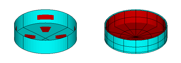
Options exist to generate three auxiliary geometry output files: gdf_pan.dat, gdf_pat.dat, and gdf_low.gdf. (Here gdf is the filename of the GDF input file. For a run with NBODY>1 the GDF filename for the first body is used.)
The files gdf_pan.dat and gdf_pat.dat contain the Cartesian coordinates of panels or patches in formats suitable for perspective plotting with programs such as Tecplot. This facilitates the use of perspective plots to illustrate and check the GDF inputs. Examples of these plots are included in Appendix A for each test run.
The file gdf_low.gdf is a low-oder GDF file, with the coordinates of new low-order panels which are derived from the input geometry. In all cases the coordinates are dimensional, and defined in the same units as specified in the input GDF file(s).
The data in gdf_low.gdf has the same definitions and format as a conventional low-order GDF file (Section 6.1). The coordinates of the panel vertices are defined with respect to the body coordinate system, corresponding to the original GDF inputs. If NBODY>1 the file gdf_low.gdf represents the body identified as N = 1. If the original body panels are reflected by the program, the file gdf_LOW.GDF will include panels for the reflected body. (This will occur if NBODY>1, if walls are present, or if the body is not symmetric with respect to the global coordinate system.) If ILOWGDF=1 and the body is reflected by the program, gdf_low.gdf contains the original body panels (without subdivision) plus their images about the reflected planes of symmetry.
The data in gdf_pan.dat and gdf_pat.dat are defined with respect to the global coordinate system. In a WAMIT run with NBODY>1 the data for all of the bodies are included. The figures in Sections A.5 and A.13 illustrate this feature.
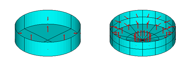
The configuration parameters IPLTNORMAL and PLTDELTA can be used to show the normal vectors on panels or patches. This may be useful to avoid errors in the direction of the normal vector, which must be directed into the interior of the body. If IPLTNORMAL=0 (default) there is no extra data to show normals. If IPLTNORMAL=1 the panels/patches are projected into the interior (or exterior if the normal is wrong). The projected patches are only shown over an interior portion of the body patch. The offset of the projected panels or patches is equal to the value of the parameter PLTDELTA, with the default value 0.05. If IPLTNORMAL=2 the normal vectors are shown at the centers of the patches or panels, and can be displayed in Tecplot using the Vector option for the zone. Examples of perspective plots using IPLTNORMAL=1 and 2 are shown in Figure 5.1 and Figure 5.2.
These files are described separately below for the low-order and higher-order methods.
In the low-order method (ILOWHI=0) the vertex coordinates of the body panels are stored in the output file gdf_pan.dat using the Tecplot finite-element format FEPOINT. The integer parameter IPLTDAT in the configuration files is used to specify whether or not to generate this output file. In the default case (IPLTDAT=0) no file is generated. If (IPLTDAT>0) the file is generated.
In the low-order method (ILOWHI=0) the optional output file gdf_LOW.GDF is controlled by the integer parameter ILOWGDF in the configuration files. If ILOWGDF> 0 the output file gdf_LOW.GDF is generated, with all of the original panels subdivided into ILOWGDF×ILOWGDF sub-divisions. The first three lines are copied from the GDF input file. The total number of sub-divided panels is included on line 4. This option can be used to increase the number of panels, and hence to increase the accuracy of the solution for the potential or source strength. However this subdivision scheme does not increase the accuracy of the geometric representation of the body, since the subdivided panels are coplanar with the original panels. Only one body can be subdivided in this manner.
In the higher-order method (ILOWHI=1) the optional output files gdf_pat.dat and gdf_pan.dat specify the vertex coordinates of both the patches and panels, as defined in Chapter 7. The integer parameter IPLTDAT in the configuration files is used to specify whether or not to generate these output files. In the default case (IPLTDAT=0) no files are generated. If (IPLTDAT>0) the number of panel subdivisions on each patch is determined by the parameters NU and NV in the SPL file, as explained in Section 7.11. If IPLTDAT=1 the data file gdf_pat.dat contains only the four vertices of each patch, and the file gdf_pan.dat contains only the four vertices of each panel. If IPLTDAT>1, each element is subdivided into IPLTDAT×IPLTDAT sub-elements. Subdivision of the elements is useful when perspective plots are constructed for bodies with curved boundaries of the patches and panels. When the curvature is large, IPLTDAT should be increased to give a more accurate plot. (IPLTDAT=5 is used for the plots shown in Sections A.11-19.)
In the higher-order method (ILOWHI=1) the format of the gdf_pat.dat file is the Tecplot ordered-list format POINT. The format of the gdf_pan.dat file depends on the configuration parameter IPLTFEPOINT. If IPLTFEPOINT=0 (default) the gdf_pan.dat file is in the Tecplot ordered-list format POINT. If IPLTFEPOINT=1 the gdf_pan.dat file is in the Tecplot finite-element format FEPOINT. If IPLTFEPOINT=1 and IPLTDAT>1 the sub-divided panels are represented in the gdf_pan.dat file.
In the higher-order method (ILOWHI=1) the optional output file gdf_LOW.GDF is controlled by the integer parameter ILOWGDF in the configuration files. If ILOWGDF> 0 a low-order GDF file is generated, using the panel vertices of the higher-order geometry with ILOWGDF×ILOWGDF sub-divisions. The first three lines are copied from the higher-order GDF input file. The total number of sub-divided panels is included on line 4. This option can be used to generate low-order GDF files for any of the geometries which can be input to the higher-order method, including geometries represented by a small number of flat patches (Section 7.5), B-splines (Section 7.6), and geometries which are defined in the subroutine GEOMXACT (Section 7.8). In each case the number of low-order panels can be increased by increasing the value of ILOWGDF. The coordinates of the panels are in the same body-fixed dimensional system as the original input data.
These optional files are generated in the POTEN subprogram, after reading the geometry input files and before looping over the wave periods. If NPER=0 these files can be generated quickly, without the extra time required to solve for the potential and hydrodynamic parameters.
5.8 ERROR MESSAGES
Numerous checks are made in WAMIT for consistency of the input data. Appropriate error messages are displayed on the monitor to assist in correcting erroneous inputs. Output files containing warning and error messages are created after each execution of the subprograms POTEN and FORCE. errorp.log contains messages from POTEN and errorf.log from FORCE. These files are overwritten with every new run. When the program runs successfully without any warning or error, the .LOG file contains two lines: a header line including the date and time when the program starts to run and a line indicating the completion of the run.
Error messages are associated with problems where the program execution is halted. Warning messages indicate that a possible error may occur, but under certain circumstances the results may be correct. Examples include failure of the convergence tests for various numerical integrations, which sometimes result from inappropriate choices of characteristic length scales or of overly conservative convergence tolerances. Another example is in the case of diffraction by a body with one or two planes of symmetry, where it is possible to compute the fluid pressures, velocities, and mean drift forces (Options 5-9) at certain heading angles without solving for all components of the diffraction potential; in this case the warning message states that the solution is non-physical, whereas at some heading angles the outputs will be correctly evaluated. For further discussion of this ‘shortcut’ see the discussion of MODE in Section 4.2 and related discussion in Section 4.3.
The same messages are displayed on the monitor during the run, and in the log file wamitlog.txt. Since some of these messages may be lost on the monitor due to scrolling of other outputs, a special warning message is generated at the end of the run to alert users when significant messages are contained in these two files.
Two particular warning messages which occur relatively frequently are the following:
- ‘Number of subdivisions exceeds MAXSQR’
- ’WARNING – no convergence in momentum Dx/Dy/Mz for headings ...’
When a warning message occurs indicating that the ‘Number of subdivisions exceeds MAXSQR’ for the Rankine integration over a higher-order panel, the Cartesian coordinates of the field point and source point are output to wamitlog.txt so that the user can more easily check if there is a singularity or inconsistency in the geometry definition in the vicinity of these points. Usually this indicates either an error in the geometry definition, or specification of a field point too close to the body surface.
The convergence test for the momentum drift force and moment is used to ensure accurate integration of the momentum flux in the far field. This integration is performed recursively, increasing the number of azimuthal integration points by factors of 2. Convergence is achieved when the difference between two successive iterations, in each of the three components Dx,Dy,Mz, is less than a prescribed tolerance TOL=10-4. If the component is less than one in absolute value, absolute differences are used, otherwise relative differences are used. The maximum number of iterations is controlled by the parameter MAXMIT in the configuration files. (With the default value MAXMIT=8 the maximum number of integration ordinates is 28 = 256.) When necessary this parameter can be increased, but it should be noted that this increases the computational time exponentially when the mean drift force and moment are evaluated from Option 8.
Since the components of the mean drift force are nondimensionalized by ULEN, and the moment by ULEN2, convergence can also be affected by the choice of ULEN in the GDF file. If ULEN is much smaller than the physical length scale of the body it will not affect the convergence tests, and vice versa. Another point to note is that some components of the force and moment may be relatively small, and of little practical importance, whereas they may affect the convergence test. When in doubt about situations where the warning message occurs, it may be advisable to increase MAXMIT by 1 or 2 units and compare the resulting outputs manually.
Starting in Version 7.0, an option can be used to issue a warning message and to output in the file wamitlog.txt all points on the body surface where the magnitude of the nondimensional fluid velocity is greater than VMAXOPT9, during the evaluation of the mean drift force and moment from pressure integration on the body surface. In this case, if VMAXOPT9≥0, data is output including the body index, panel or patch index, location of the point in dimensional body coordinates, and magnitude of the fluid velocity. The parameter VMAXOPT9 may be included in the configuration file (cfg), as explained in Section 3.7. The default value VMAXOPT9=-1.0 is assigned if there is no input, with the result that the above warning and outputs are not included. This option can only be used if IOPTN(9)>0 in the Force Control File. This option can be used to identify points where the representation of the body geometry is deficient in such a way that the evaluation of the fluid velocity is non-physical. In general the fluid velocity should be of order of magnitude one, or smaller, on the body surface, and values which are much greater than this may be due to either sharp corners (which are physically correct) or defects in the representation of the body geometry (which are not physically correct). This option should be used with care, to avoid excessive outputs. If VMAXOPT9=0.0, every integration point will be output, for all wave periods, heading angles, and symmetry planes of the body.
5.9 THE LOG FILE (wamitlog.txt)
The file wamitlog.txt is output during the run to provide an archival record. The file includes the starting and ending time and date for each sub-program, copies of the principal input files, and copies of the outputs in the files errorp.log and errorf.log. (Since the GDF input files are relatively long in the low-order method, and also in the higher-order method when the geometry is defined by low-order panels or B-splines, only the first 10 lines of the GDF file are copied in these cases. The maximum width of lines of data is truncated to 80 characters in wamitlog.txt. The existing wamitlog.txt file, in the directory where the program runs, is overwritten with every new run. If IOUTLOG=1 is assigned, the file wamitlog.txt is copied at the end of the run to a second file with the same filename as the OUT files, ending in _log, to provide an archive of the inputs for the run. Otherwise, if it is appropriate to save this file, it should be renamed or moved to a directory where it is protected.
When the input data in the FRC file is in the Alternative form 1, as described in Section 4.3, the nondimensional inertia matrix for each body is included in the file wamitlog.txt. This is useful when the analysis of a body is first performed using Alternative form 1, and then changed for subsequent extensions to Alternative form 2, for example when external damping is imposed on an otherwise freely floating body. The normalizing factors for the nondimensional inertia matrix are the products of the fluid density and appropriate powers of the characteristic length parameter ULEN. In preparing a force control file for Alternative form 2, as described in Section 4.4, these normalizing factors must be included in the inputs EXMASS when these are derived from the nondimensional inertia matrix.
5.10 THE INTERMEDIATE DATA TRANSFER FILE (P2F)
The file pot.p2f is written by POTEN and read by FORCE. The filename pot is the same as the POT input file. The P2F file contains the solutions of the linear systems of equations for the velocity potential (and source strength) on the body surface, and also some inputs to POTEN which are required by FORCE, e.g. the wave periods and heading angles specified in the POT file. To facilitate data transfer the P2F file is a binary file, and it cannot be used for purposes other than as input to FORCE.
The P2F file can be used for multiple runs of FORCE, in situations where the outputs from POTEN are the same. TEST07b and TEST17b are examples of this situation, where the only change from TEST07a or TEST17a is to apply an external damping force to attenuate the roll damping or moonpool resonance. IPOTEN=0 is assigned in the configuration file and the POTEN run is skipped, with considerable savings of time. Increasing the number of Haskind wave heading angles, adding options in FRC which were omitted in the original run, and using an external RAO file (Section 4.13) are examples of other situations where it is useful to save the original P2F file and avoid the extra computational time required to repeat the POTEN run.
If another run is made using the same POT file, with IPOTEN=1 (default) and with an old P2F file in the same directory with the same filename, the user is interrogated with options to over-write the old P2F file or to assign a different name to the new file. This interruption can be avoided by renaming or deleting the old P2F file, or using the configuration parameter IDELFILES as explained in Section 4.7.
The P2F files can be relatively large, depending on the parameters of the run. Unless future use is anticipated it may be best to erase or over-write old files.