Chapter 15
THEORY
In this Chapter the theoretical basis for WAMIT is described. Further information can be found in Reference [26], and in the references cited below.
15.1 THE BOUNDARY-VALUE PROBLEM
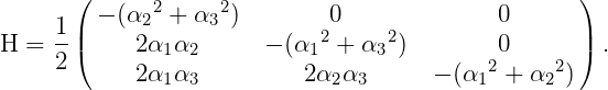
A three-dimensional body interacts with plane progressive waves in water of finite depth H. The objective of WAMIT is to evaluate the unsteady hydrodynamic pressure, loads and motions of the body, as well as the pressure and velocity in the fluid domain. The flow is assumed to be potential, free of separation or lifting effects. The free-surface and body-boundary conditions are linearized. A harmonic time dependence is adopted.
The Cartesian coordinate system (x,y,z) is defined as shown in Figure 4.1, fixed relative to the undisturbed positions of the free surface and body with the z-axis positive upwards. The body geometry input to WAMIT is defined relative to the body coordinate system and the incident-wave system is defined relative to the global coordinates, as explained in Chapter 3 and Section 4.2. For the sake of simplicity here it is assumed that these two coordinate systems coincide.
The assumption of a potential flow permits the definition of the flow velocity as the gradient of the velocity potential Φ satisfying the Laplace equation
 | (15.1) |
in the fluid domain. The harmonic time dependence allows the definition of a complex velocity potential φ, related to Φ by
 | (15.2) |
where Re denotes the real part, ω is the frequency of the incident wave and t is time. The ensuing boundary-value problem will be expressed in terms of the complex velocity potential φ, with the understanding that the product of all complex quantities with the factor eiωt applies. The linearized form of the free-surface condition is
 | (15.3) |
Here K = ω2∕g is the infinite-depth wavenumber and g is the acceleration of gravity. The velocity potential of the incident wave is defined by
![φ0 = igA--cosh-[k(z-+-H-)]e-ikxcosβ- ikysinβ,
ω coshkH](images/wamit_v74manual80x.png) | (15.4) |
where the wavenumber k is the real root of the dispersion relation
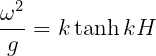 | (15.5) |
and β is the angle between the direction of propagation of the incident wave and the positive x-axis as defined in Figure 4.1. In the limiting case of infinite depth k = K. To distinguish these two parameters, they are referred to as the ‘finite-depth’ and ‘infinite-depth’ wavenumbers, respectively. The wavelength is equal to 2π∕k and the wave period is equal to 2π∕ω.
The linearization of the problem permits the decomposition of the velocity potential φ into the radiation and diffraction components
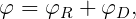 | (15.6) |
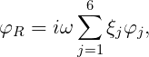 | (15.7) |
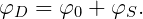 | (15.8) |
The constants ξj denote the complex amplitudes of the body oscillatory motion in its six rigid-body degrees of freedom, and φj the corresponding unit-amplitude radiation potentials. The velocity potential φS represents the scattered disturbance of the incident wave by the body fixed at its undisturbed position. We will refer to the sum (15.8) as the diffraction potential φD.
On the undisturbed position of the body boundary, the radiation and diffraction potentials are subject to the conditions,
 | (15.9) |
 | (15.10) |
where (n1,n2,n3) = n and (n4,n5,n6) = x × n, x = (x,y,z). The unit vector n is normal to the body boundary and points out of the fluid domain.
The radiation condition of outgoing waves in the far field is applied to the velocity potentials φj, j = 1,…, 7.
15.2 INTEGRAL EQUATIONS FOR THE VELOCITY POTENTIAL
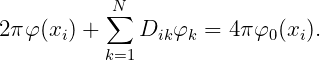
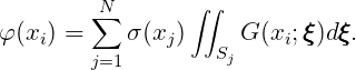
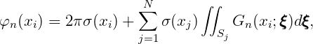
In WAMIT the boundary value problems defined above are solved by using Green’s theorem to derive integral equations for the radiation and diffraction velocity potentials on the body boundary. The integral equation satisfied by the radiation velocity potentials φj on the body boundary takes the form
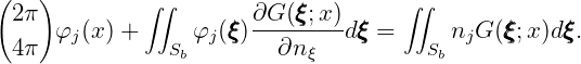 | (15.11) |
Here Sb denotes the wetted surface of the body, in its fixed mean position, on or below the plane z = 0. If Sb is entirely below z = 0 (except for the waterline intersection) the factor 2π applies at all points on Sb. In special cases where part or all of Sb is in the plane z = 0 the factor 4π applies for points where z = 0 and 2π applies if z < 0. These special cases are not considered hereafter, except in Section 15.13.
The corresponding equation for the total diffraction velocity potential φD is
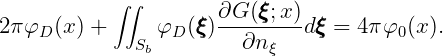 | (15.12) |
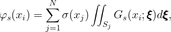
The diffraction potential may also be obtained from equation (15.8) after solving for the scattered potential φS. The equation for the scattered velocity potential is
 | (15.13) |
From the computational point of view, equation (15.12) has some advantages over (15.13) in terms of cpu time and the requirement of storage space, because of the relative simplicity of the right-hand side.
The Green function G(x;ξ ξ ξ) is referred to as the wave source potential. It is the velocity potential at the point x due to a point source of strength -4π located at the point ξ ξ ξ. It satisfies the free-surface and radiation conditions, and in infinite water depth is defined by
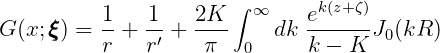 | (15.14) |
 | (15.15) |
 | (15.16) |
where J0(x) is the Bessel function of zero order. In finite depth, the Green function is defined by
 | (15.17) |
 | (15.18) |
In both expressions (15.14) and (15.17) the Fourier k-integration is indented above the pole on the real axis in order to enforce the radiation condition. Efficient algorithms for the evaluation of the infinite and finite-depth wave-source potentials and their spatial derivatives, have been developed in [1] and [11].
Special attention must be given to the singular components of the Green function for small values of r,r′ and r′′. The source-like singularities 1∕r, 1∕r′ and 1∕r′′ and their normal derivatives can be integrated analytically over a quadrilateral panel, as described in [2]. In addition, the ascending series expansion of the wave source potential for small values of r′ (Ref. [1], eq.(5)), reveals the presence of the logarithmic singularity,
 | (15.19) |
(The derivation of this result in [1] is for the infinite-depth case, but it can be shown from the analysis of the finite-depth case in the same reference that the same singularity applies.) Provision has been made in WAMIT to permit the logarithmic singularity and its derivatives to be integrated analytically in the solution of the integral equations when the source and field points are close to each other and to the free surface. Further details are given in Section 15.3.
15.3 DISCRETIZATION OF THE INTEGRAL EQUATIONS IN THE LOW-ORDER METHOD (ILOWHI=0)
The mean position of the body wetted surface is approximated by a collection of quadrilaterals. Each quadrilateral is defined by four vertices, lying on the body surface. Their Cartesian coordinates are input to WAMIT. They are numbered in the counter-clockwise direction when the panel is viewed from the fluid domain. Instructions on how to input the vertex coordinates are given in Chapter 6.
In general the quadrilaterals defined above are not plane, but if a sufficiently fine discretization is used for a boundary surface with continuous curvature, each element will approach a plane surface. In this circumstance a plane approximation of the general quadrilateral is defined by the midpoints of each side, which always lie in the same plane. Each panel is defined by projecting the four vertices onto this plane. If the coordinates of two adjacent vertices coincide, the quadrilateral panel reduces to a triangular panel.
For bodies of general shape, gaps may exist between panels. Experience suggests that they do not significantly affect the accuracy of the velocity potential and the hydrodynamic forces.
The radiation and diffraction velocity potentials are taken to be constant over each panel. The discretization errors associated with the selection of plane panels and a piecewise constant variation of the velocity potential are of the same order, if the integration of the singular components of the wave source potential over the panels are carried out with sufficient accuracy.
Based on this discretization, the continuous integral equations (15.11) and (15.12) can be reduced to a set of linear simultaneous equations for the values of the velocity potentials over the panels. For the radiation potentials we obtain
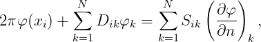 | (15.20) |
where i = 1,…,N, N being the number of panels. For the total diffraction potential
 | (15.21) |
The matrices Dik and Sik are defined by
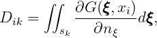 | (15.22) |
 | (15.23) |
where sk denotes the surface of the k-th panel. The ‘collocation’ points xi, where the integral equations are enforced, are located at the panel centroids.
The analytic integration of the Rankine source potentials and their derivatives follows the theory outlined in [2]. The formulae used for the analytic integration of the logarithmic singularity are derived in [6]. The integration over each panel of the regular part of the wave source potential is approximated by multiplying the value of the integrand at the centroid by the panel area.
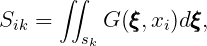
15.4 INTEGRAL EQUATIONS FOR THE SOURCE FORMULATION
In the low-order method the source formulation is used to derive the fluid velocity components on the body surface. The velocity potential is expressed by a distribution of sources only, in the form
 | (15.24) |
After discretizing the body surface with plane panels, with constant source strength on each panel, the potential is expressed by
 | (15.25) |
Denote the normal vector as  and the two tangential unit vectors as
  and
and  on each panel.
The three components of the velocity are then given in the (
on each panel.
The three components of the velocity are then given in the ( ,
, ,
, ) coordinate system as
follows:
) coordinate system as
follows:
 | (15.26) |
 | (15.27) |
 | (15.28) |
15.5 DISCRETIZATION OF THE INTEGRAL EQUATIONS IN THE HIGHER-ORDER METHOD (ILOWHI=1)
The mean body surface is defined by ‘patches’, as explained in Chapter 7. Each patch must be a smooth continuous surface. The Cartesian coordinates x = (x,y,z) of a point on the patch are expressed in term of two parametric coordinates u = (u,v). These are normalized so that they vary between 1 in the domain of the patch. Details of the geometric description of the body surface are provided in Chapter 7.
The velocity potential on each patch is represented by a product of B-spline basis functions U(u) and V (v) as shown in equation (7.4). The total number of B-spline basis functions on each patch is Mu times Mv.
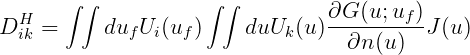
Upon substituting equations (7.3) and (7.4), (15.11) can be expressed in the form
where, Uk = Ul(u)V m(v), ∫ ∫ du = ∫ -11dv∫ -11du, J(u) is Jacobian and N p denotes the number of patches.
Following the Galerkin method, (15.29) is multiplied by Ui and integrated over each patch. This results in the linear system
 | (15.30) |
for the radiation potential. Similarly, from (15.12), we obtain
 | (15.31) |
for the diffraction potential.
In the above equations, (ϕj)k and (ϕD)k are unknown coefficients of basis function for the radiation and diffraction potentials, respectively. The matrices dikH and D ikH and vectors S iH and IiH are defined by
 | (15.32) |
 | (15.33) |
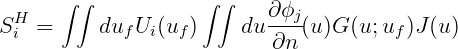 | (15.34) |
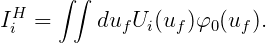 | (15.35) |
As explained in Chapter 7, a set of B-spline basis functions is defined by the order of the polynomial (Ku and Kv) and the number of panels (Nu and Nv). In general, the basis function has nonzero value over a part of the patch. For example, Ul(u)V m(v) is nonzero on the panels from l - Ku + 1- (or 1, if l - Ku + 1 < 1) to l-th panels (or Nu, if l > Nu) in u and m - Kv + 1- (or 1, if m - Kv + 1 < 1) to m-th (or Nv, if m > Nv) panels in v.
The integration in uf over each panel is referred to as the ‘outer’ integration. This is carried out by Gauss-Legendre quadrature. The order of the quadrature is specified by the input parameters IQUO and IQVO in the SPL file, for u and v respectively, or by the parameter IQUADO in the configuration files. The order of the basis functions are specified by the parameters KU and KV in the SPL file, or KSPLIN in the configuration files.
The inner integrations in u in equations (15.33) and (15.34) are carried out as described below, for each abscissa of the Gaussian quadrature for the outer integral, uf.
The integration of the regular part of the wave source potential is carried out by Gauss-Legendre quadrature. The order of the inner quadrature is specified by the input parameters IQUI and IQVI in the SPL file or by the parameter IQUADI in the configuration files. Numerical tests suggest that the order of the quadratures should be one order higher than the order of the basis functions.
The integrals involving the Rankine source and normal dipole are evaluated in the manner explained next. If the field point uf is on the panel, the integrand is singular at this point. Otherwise the integrand is regular throughout the domain of the panel. In the singular case, the panel is subdivided into a small square subdomain centered at uf, and one or more rectangular subdivisions adjoining the square as required to cover the remainder of the panel. The integrals over the latter subdivisions are treated in the same manner as for the other panels where the integrand is regular.
The integrals where the integrand is regular are evaluated by Gauss-Legendre quadrature. If
the field point is near the panel, the panel is subdivided into four smaller panels. This
subdivision is repeated until the size of the subdivided panel is less than a prescribed multiple of
the physical distance from uf to the centroid of the panel. For this purpose the size of the panel
is defined as the maximum physical length from the center of the panel to its four vertices. The
maximum size permitted without further subdivision is 1∕ = 2∕3. In some cases a large
number of subdivisions are required, particularly when uf is close to the sides or vertices
of the panel. In this case, the program terminates subdivision after the domain is
subdivided into 2048 subdomains. The program issues a warning message to the monitor
and error log file but continues without interruption. This warning message is most
likely to occur when the mapping of a physical surface onto a patch is singular, as
at the poles of a spherical or spheroidal surface, and the accuracy of most relevant
hydrodynamic outputs are not affected significantly by this problem. In other cases the warning
message may be an indication that the geometrical representation of the body surface is
defective.
= 2∕3. In some cases a large
number of subdivisions are required, particularly when uf is close to the sides or vertices
of the panel. In this case, the program terminates subdivision after the domain is
subdivided into 2048 subdomains. The program issues a warning message to the monitor
and error log file but continues without interruption. This warning message is most
likely to occur when the mapping of a physical surface onto a patch is singular, as
at the poles of a spherical or spheroidal surface, and the accuracy of most relevant
hydrodynamic outputs are not affected significantly by this problem. In other cases the warning
message may be an indication that the geometrical representation of the body surface is
defective.
The singular integral over the square subdomain centered at uf is explained below. The integration of the dipole is defined in the ‘principal-value’ sense excluding a vanishingly small area around the origin. With this definition for the dipole integral, both the source and dipole distributions can be evaluated in the same manner.
After an appropriate normalization of the length and use of local coordinates with the origin at (uf,vf), the integral takes the form
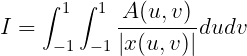 | (15.36) |
where A(u,v) is regular function. |x(u,v)| is the distance between the source and field points in physical space.
For simplicity, we consider only the case where |∂x
∂u| = 1, |∂x
∂v| = 1 and ∂x
∂u ⋅ ∂x
∂v = 0 but the
analysis below can be applied directly to the general case. Since |x|∕ is regular and thus
(15.36) can be expressed in the form
is regular and thus
(15.36) can be expressed in the form
 | (15.37) |
where f(u,v) is regular.
The singularity at the origin is removed by subdividing the square domain into 4 isosceles triangles with a common vertex at the origin and evaluating the integral separately over each triangle. For example, the integral over a triangle with a side on u = 1 is
 | (15.38) |
After the change of variables u = p, v = pq, we have
 | (15.39) |
After adding the contributions from other three triangles, we have
 | (15.40) |
Next we remove the square-root function from (15.40). By change of the variables q = sinh(as), we have
 | (15.41) |
where a = sinh-11. The integral (15.41) is evaluated by applying the Gauss-Legendre quadrature in p and s coordinates.
The integral of the log singularity in the free-surface component of the source potential can be evaluated either in a similar manner as for the Rankine source, or together with the regular part of the wave source potential. The parameter ILOG in the configuration files controls these options. When ILOG=1, the logarithmic singularity is subtracted from the wave-source potential and integrated separately. When ILOG=0 it is included in the evaluation of the wave-source potential and integrated by the same quadrature.
15.6 REMOVAL OF IRREGULAR FREQUENCIES
The irregular frequency effects are removed from the velocity potential and the source strength using the extended boundary integral equations. The details of discussion on the method are provided in Reference [8] and [16].
The extended boundary integral equation for the potential formulation (15.11) takes a form
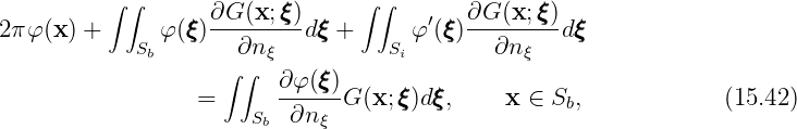
Here φ(x) is the unknown velocity potential on the body surface Sb and φ′(x) is the nonphysical velocity potential on the interior free surface Si.
The corresponding equations for the source formulation (15.26) are
 | (15.44) |
 | (15.45) |
15.7 INTEGRAL EQUATIONS FOR BODIES WITH THIN SUBMERGED ELEMENTS
Green’s integral equations in Section 15.2 become singular as the thickness of the body (or part of the body) decreases. To avoid this singularity in the discretized problem, the panel size should be of the same order as the thickness, or smaller, in order to render the linear system well-conditioned. Thus the size of the linear system becomes large as the thickness decreases.
An alternative form, which is nonsingular, can be obtained from Green’s integral equation for the limit when the thickness is zero. In this modified form of the integral equation, the velocity potential is represented by a distribution of dipoles only, without sources. The dipole strength is equal to the difference of the velocity potential on two opposite sides of the zero-thickness surface, denoted by Δϕ below.
If the body surface Sb consists partly of thin ‘dipole’ elements Sd and partly of conventional ‘source’ elements Ss which are represented by both sources and dipoles, Green’s integral equations (15.11-13) and the dipole distribution can be combined in the following form:
 | (15.46) |
when x is on the conventional body surface Ss, and
 | (15.47) |
when x is on the surface of zero thickness Sd. In the diffraction problem for the potential ϕD, the right-hand-side of (15.46) and (15.47) are replaced by 4πφ0(x) and 4πφ0n(x).
Instructions for using this option are in Sections 6.3 and 7.10. TEST09 and TEST21, described in Appendix A, are examples of its use.
It should be emphasized that thin dipole elements must be submerged, in contact with the fluid on both sides. A thin element which is in the plane of the free surface, and only in contact with the fluid on the lower side, should be considered as part of the conventional surface Ss.
15.8 MEAN DRIFT FORCES BASED ON PRESSURE INTEGRATION
The instantaneous position vector ( ) in an inertial coordinate system of the point fixed on
the body fixed coordinate system (
) in an inertial coordinate system of the point fixed on
the body fixed coordinate system ( ) is given by
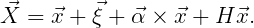 | (15.48) |
For the present purpose we consider only the first order quantities of the translational modes  ,
the rotational modes
,
the rotational modes  and the velocity potential ϕ. The roll-pitch-yaw sequence of rotations is
adopted, and the transformation matrix is given by
and the velocity potential ϕ. The roll-pitch-yaw sequence of rotations is
adopted, and the transformation matrix is given by
 | (15.49) |
The normal vector in the inertial coordinate system can be expressed by
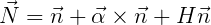 | (15.50) |
where  is the normal vector on the body boundary in the body fixed coordinate
system.
is the normal vector on the body boundary in the body fixed coordinate
system.
The pressure at the instantaneous position  given in the equation (15.48) can be expressed
by
given in the equation (15.48) can be expressed
by
where Zo is the vertical coordinate of O relative to the free-surface.
![P = - ρ[g(z + Zo) + (ϕt + g(ξ3 + α1y - α2x ))
+ (1∇ ϕ ⋅ ∇ ϕ + (⃗ξ + ⃗α × ⃗x) ⋅ ∇ ϕ + gH ⃗x ⋅ ∇z )] (15.51)
2 t](images/wamit_v74manual141x.png)
The mean forces and moments are obtained by time averaging the following expressions for the forces and moments:
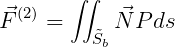 | (15.52) |
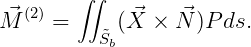 | (15.53) |
In equations (15.52) and (15.53), the integrations are over the exact body wetted surface
 b.
b.
After substituting (15.48), (15.50), and (15.51) and integrating the hydrostatic components,
![(2) 1- ∫ ′ 2
⃗F = 2 ρg WL ⃗n [ζ - 2ζ(ξ3 + α1y - α2x )]dl
1 ∫ n
+ --ρg⃗k ∘----z---[ζ - (ξ3 + α1y - α2x )]2dl
2 W L 1 - n2z
∫∫
- ρ ⃗n( 1∇ ϕ ⋅ ∇ ϕ + (⃗ξ + α⃗× ⃗x) ⋅ ∇ϕt)ds
Sb 2∫∫
+ ⃗α × (- ρ Sb ⃗nϕtds )
⃗(2)
+ F S (15.54)](images/wamit_v74manual145x.png)
![⃗ (2) 1- ∫ ′ 2
M = 2ρg W L(⃗x × ⃗n )[ζ - 2ζ(ξ3 + α1y - α2x )]dl
1 ∫ n
+ -ρg ∘----z---(⃗x × ⃗k)[ζ - (ξ3 + α1y - α2x )]2dl
2 W L 1 - n2z
∫∫ 1
- ρ (⃗x × ⃗n)(--∇ ϕ ⋅ ∇ ϕ + (ξ⃗+ ⃗α × ⃗x) ⋅ ∇ ϕt)ds
Sb∫∫ 2
- ρ⃗α × (⃗x × ⃗n)ϕ ds
Sb t
∫∫
+ ⃗ξ × (- ρ ⃗nϕtds )
(2) Sb
+ ⃗M S (15.55)](images/wamit_v74manual146x.png)
where the hydrostatic components are
![(2) { }
⃗FS = - ρgAwp α1α3xf + α2 α3yf + 12(α21 + α22)Zo ⃗k (15.56)
(2) {
M⃗S = ρg [(ξ2α2 - ξ3α3 )Awpxf - ξ2α1Awpyf + α1 α2Awpxf Zo
3 2 1 2
- (2α1 + 2α 2)Awpyf Zo - ξ2ξ3Awp - ξ3α1AwpZo
+ α α (L - L ) - 2α α L + α α ∀x - 1(α2 + α2)∀y ]⃗i
2 3 11 22 1 3 12 1 2 b 2 1 3 b
[- ξ1α2Awpxf + (ξ1α1 - ξ3α3 )Awpyf + (12α21 + 32α22)Awpxf Zo
- α α A y Z + ξ ξA - ξ α A Z + α α (L - L )
1 2 wp f o 1 3 wp 3} 2 wp o 1 3 11 22
+2 α2α3L12 + 1(α2 + α2)∀xb]⃗j . (15.57)
2 2 3](images/wamit_v74manual147x.png)
Here ζ is the first order runup, Awp is the waterplane area and ∀ is the volume of the body.
In addition (xf,yf) are the coordinates of the center of flotation, (xb,yb,zb) are the
coordinates of the center of buoyancy, ( ,
, ,
, ) are positive unit vectors relative to
the x,y,z coordinates, and Lij = ∫
wpxixjds denotes the moments of the waterplane
area.
) are positive unit vectors relative to
the x,y,z coordinates, and Lij = ∫
wpxixjds denotes the moments of the waterplane
area.
15.9 MEAN DRIFT FORCES USING CONTROL SURFACES
The mean drift force and moment are evaluated by one the following two alternatives depending on the value of IALTCSF in the CFG file.
IALTCSF=1:
![∫ ∫
⃗F (2) = - 1ρg ⃗n′ζ2dl - ρg ⃗k ζ[(ξ⃗+ ⃗α × ⃗x) ⋅⃗n ′]dl
2 CL W L
1 ∫ nz 2
+ 2ρg ⃗k ∘------2[ζ - (ξ3 + α1y - α2x)] dl
W L 1 - nz
∫ ∫ ∂ϕ 1
- ρ [∇ ϕ ---- -⃗n(∇ ϕ ⋅ ∇ ϕ)]ds
∫S∫c ∂n 2
+ ρ⃗k (ζ∂-ϕt+ 1∇ ϕ ⋅ ∇ ϕ)ds + ⃗F (2) (15.58)
Sf ∂z 2 S](images/wamit_v74manual151x.png)
dl
2 ∫CL W L
1- ∘--nz---- ⃗ 2
+ 2ρg W L 1 - n2 (⃗x × k)[ζ - (ξ3 + α1y - α2x )]dl
∫∫ z
∂-ϕ 1-
- ρ Sc[(⃗x × ∇ ϕ)∂n - 2(⃗x × ⃗n )(∇ϕ ⋅ ∇ ϕ )]ds
∫∫ ∂ϕ 1
+ ρ (⃗x × ⃗k )(ζ --t-+ --∇ ϕ ⋅ ∇ ϕ)ds + ⃗M (S2) (15.59)
Sf ∂z 2](images/wamit_v74manual152x.png)
IALTCSF=2:
![∫ ∫ ∫
⃗F(2) = 1-ρg ⃗n′ζ2dl - ρg ζ∇ ′ζds
2 WL Sf
∫ ′
- ρg⃗k ζ[(⃗ξ + ⃗α × ⃗x ) ⋅⃗n ]dl
W∫L
+ 1-ρg⃗k ∘--nz----[ζ - (ξ3 + α1y - α2x )]2dl
2 W L 1 - n2z
∫∫
- ρ [∇ ϕ∂-ϕ - 1⃗n (∇ ϕ ⋅ ∇ϕ )]ds
Sc ∂n 2
∫∫ ∂ϕt 1 (2)
+ ρ⃗k (ζ ----+ --∇ ϕ ⋅ ∇ϕ )ds + ⃗FS (15.60)
Sf ∂z 2](images/wamit_v74manual153x.png)
dl
W∫L
+ 1ρg ∘--nz----(⃗x × ⃗k)[ζ - (ξ3 + α1y - α2x )]2dl
2 W L 1 - n2z
∫ ∫
- ρ [(⃗x × ∇ ϕ)∂-ϕ - 1-(⃗x × ⃗n)(∇ ϕ ⋅ ∇ϕ )]ds
Sc ∂n 2
∫ ∫ ∂ϕt 1 (2)
+ ρ (⃗x × ⃗k)(ζ----+ -∇ ϕ ⋅ ∇ ϕ)ds + ⃗M S (15.61)
Sf ∂z 2](images/wamit_v74manual154x.png)
In these equations Sc is the submerged part of the control surface, Sf is the part of the
control surface on the free surface, WL is the body waterline and CL is the common boundary of
Sc and Sf.  ′ denotes the two-dimensional normal vector in the horizontal plane on the body
waterline, pointing into the body, ∇′ is the gradient in the horizontal plane, and
′ denotes the two-dimensional normal vector in the horizontal plane on the body
waterline, pointing into the body, ∇′ is the gradient in the horizontal plane, and  is the unit
vector pointing vertically upward.
is the unit
vector pointing vertically upward.  S(2) and
  S(2) are the hydrostatic components (15.56-15.57).
The derivations of the equations (15.58-15.61) from (15.54-15.55) are given in Reference [28].
S(2) are the hydrostatic components (15.56-15.57).
The derivations of the equations (15.58-15.61) from (15.54-15.55) are given in Reference [28].
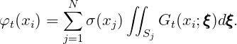
15.10 INTERNAL TANK EFFECTS
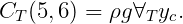
The solution for the velocity potential in each tank, and the resulting forces and moments, are computed in a similar manner as for the exterior domain outside the body or bodies. Since there is no diffraction potential to consider, the velocity potential ϕ in each tank is
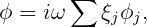 | (15.62) |
and the first-order pressure at a fixed point on the tank surface is given by
 | (15.63) |
Here ZT is the vertical coordinate of the tank free surface above the origin.
The solution for the velocity potential ϕ in each tank is computed simultaneously with the potential in the exterior fluid domain outside the hull, using one extended linear system which includes all of the fluid domains (exterior plus interior of all tanks). The principal modification is to impose the condition that there is no influence between the separate fluid domains. Thus the elements in the extended influence coefficient matrix are set equal to zero if the row and column correspond to different domains. Further details are given in Reference [27].
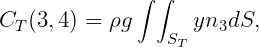
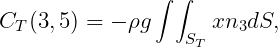
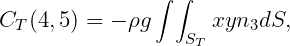
The force and moment exerted by the tank fluid on the vessel are given by
 | (15.64) |
 | (15.65) |
where n is the normal pointing out of the tank (away from the fluid domain of the tank) and double integrals are over the submerged surface of the tank.
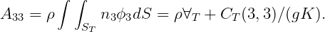
After some vector analysis these equations give relations similar to (15.52-15.53) for the contributions from the hydrostatic pressure:
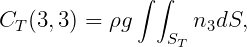

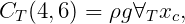

All other elements of the matrix CT are equal to zero. Here
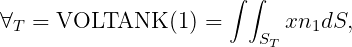
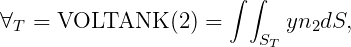
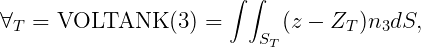
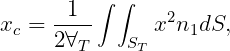
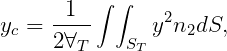
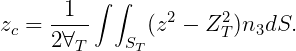
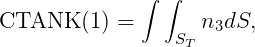
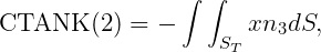
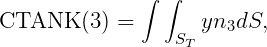
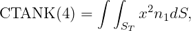
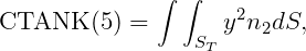
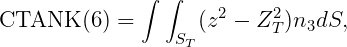
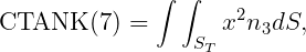
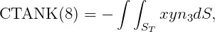
In WAMIT the hydrostatic parameters of the hull and tanks are evaluated separately. Thus VOL, C(i,j) are evaluated for the hull ignoring tank patches/panels and their values are the same with or without tanks, as defined in Section 3.1. The corresponding tank parameters VOLTNK(1:3,1:NTANK) and CTANK(1:9,1:NTANK) are evaluated separately for each tank (the second index is omitted for simplicity of notation):

It is necessary to consider the implications of planes of symmetry with respect to the tanks. If all of the tanks are symmetric about a plane of symmetry, then it is appropriate to use that option (assuming the hull is also symmetric about the same plane). Thus, for example, for a hull with symmetry about y=0, and with all tanks symmetric about the same plane, it is appropriate to set IS(2)=1. But if there are two or more tanks along the x-axis, IS(1)=0 is required. When planes of symmetry are appropriate, the following integrals (which are originally evaluated over one half or one quarter of the tank, with nonzero values), should be set equal to zero:
If IS(1)=1, CTANK(2) = 0, CTANK(4) = 0, CTANK(8) = 0,
If IS(2)=1, CTANK(3) = 0, CTANK(5) = 0, CTANK(8) = 0.
All other elements are multiplied by IMUL=2 or 4 to account for the planes of symmetry, in the same manner as C(I,J).
In GETIF, after CALL OPHEAD to output the hydrostatic matrix for the hull, the subroutine TANKFS is called when tanks are present. In TANKFS the following assignments are made for the hydrostatic restoring coefficients, where the extra terms added for the tanks are summed over all tanks associated with each body:


![C (4, 4) = C(4,4) + (ρ ∕ρ )[CTANK (9) - 1CTANK (6)]
T 2](images/wamit_v74manual189x.png)

![[ ]
C (5,5) = C (5,5) + (ρ ∕ρ) CTANK (7) - 1CTANK (6) .
T 2](images/wamit_v74manual191x.png)
Also, if IALTFRC=2,


The extra terms in C(4, 6) and C(5, 6) are omitted for a freely-floating body since these are balanced by the vessel’s corresponding buoyancy moments.
When tanks are present, the header of the output file frc.out includes nondimensional values of the tank volumes and the contributions from the tanks to C(3, 3), C(3, 4) and C(3, 5).
Next consider the inertia forces and moments due to the body mass. If IALTFRC=1 the body mass m is calculated from VOL and all of the inertia coefficients are propotional to m. Since VOL is the total displaced volume of the hull, the static mass of the fluid in the tanks is included in m. However the same inertia effects are represented (more correctly for dynamic conditions) by the added mass of the tank, to be discussed below. For this reason, if IALTFRC=1, the mass matrix is reduced by the sum ∑ (ρT ∕ρ)×VOLTANK/VOLM, where the sum is over all tanks. Likewise, the terms -mgzg in the restoring coefficients C(4, 4) and C(5, 5) are reduced. If IALTFRC=2 these corrections are not made, and the external mass matrix should exclude the fluid in the tanks. If IALTFRC=1 the radii of gyration should be estimated ignoring the fluid in the tanks.
The added mass and damping coefficients are evaluated globally, by integrating the corresponding components of the pressure over both the external hull surface and the internal tank surfaces. The only modification for tank panels/patches is to multiply their contributions by RHOTANK, the relative density of the tank fluid compared to the external fluid. Since there is no radiation from the tanks, the damping coefficients should be zero. In test calculations they are generally very small, except near tank resonances. (A useful check is to verify that the damping coefficients of the hull with tanks are equal to the damping coefficients without tanks.)
Special attention is required for the vertical modes (heave, roll, pitch), where there is a fictitious hydrostatic contribution to the added mass. First consider heave, where the relevant boundary conditions are ϕn = n3 on Sb and Kϕ - ϕz = 0 on the free surface. Here K = ω2∕g. Thus the heave potential is given by ϕ 3 = z + 1∕K, where z is a local vertical coordinate with its origin in the tank free surface. The heave added-mass coefficient is
 | (15.66) |
 | (15.67) |
 | (15.68) |
Since ω2 = gK, the last terms are cancelled by the hydrostatic restoring coefficients. Thus, in the limit ω → 0, there are no contributions to the equations of motion for the LHS elements associated with the vertical force or vertical translation, as expected on physical grounds.
In the classical hydrostatic analysis of ships, the tank free-surface effect is evaluated by considering the second moments of the tank free surface about a local origin at the centroid of the free surface, whereas in the expressions for CT these moments are about the global origin. This difference can also be explained in terms of the corresponding added mass coefficients, in an analogous manner to the analysis above.
15.11 BODIES WITH PRESSURE SURFACES
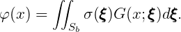
The boundary-value problem described in Section 15.1 is extended here to include problems where part or all of the body surface is one or more free surfaces, and a nonzero oscillatory pressure acts on these surfaces. On each of these surfaces the hydrostatic pressure is assumed constant, and non-negative. Thus the surface is in a horizontal plane at z ≤ 0. The oscillatory component of the pressure is defined as the real part of p0(x,y)eiωt. The complete boundary surface Sb = Sw + Sp includes the ‘wetted’ surface Sw and the ‘pressure’ surface Sp. To simplify the notation it is assumed here that NBODY=1 and there are no generalized modes. The Neumann boundary conditions (15.9) and (15.10) are applicable on Sw, and the boundary condition on Sp is
 | (15.69) |
It is convenient to represent the pressure distribution by
 | (15.70) |
where, for j > 6, ξj is a normalized coefficient with the dimension of length and nj is a nondimensional real function of position which represents the spatial dependence of the corresponding pressure mode. The number of modes Mp required to represent the pressure distribution will depend on the application. The total potential is given by (15.6), with the radiation potential extended in the form
 | (15.71) |
If the functions nj are extended to apply on both Sb and Sp, with the definitions

 | (15.72) |
where
When necessary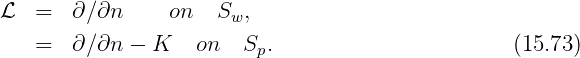
 x and ξ will be used to indicate that the normal derivative is with respect to
the corresponding coordinates.
x and ξ will be used to indicate that the normal derivative is with respect to
the corresponding coordinates.
The integral equation (15.11) for the velocity potential is replaced by
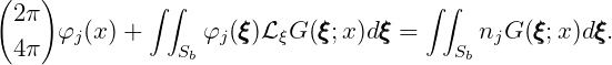 | (15.74) |
The factor 2π is applied if the boundary surface is below z = 0, and 4π is applied if the boundary surface is on z = 0. In the latter case the integral over Sp on the left-hand-side of (15.74) vanishes, since the Green function satisfies the homogeneous free-surface condition. In the source formulation, where the potential is given by (15.24), the integral equation corresponding to (15.26) is
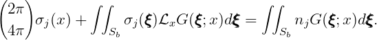 | (15.75) |
In the diffraction problem the potential (15.8) satisfies the integral equation
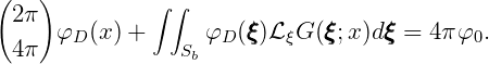 | (15.76) |
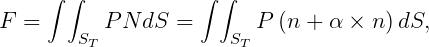
The definitions of the added-mass and damping coefficients in the first equation of
Section 3.2 are unchanged, except for the extended range of the subscripts (i,j). In the
definition of the Haskind exciting forces in Section 4.3 the normal derivative of the
incident-wave potential is replaced by φ0. The definition of the exciting forces from
direct integration of pressure is given by the second equation in Section 3.3, without
change.
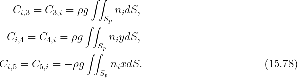
The definitions of the hydrostatic restoring coefficients Cij for (i,j) ≤ 6 are unchanged, as given in Section 3.1. The restoring coefficients for (i,j) ≥ 7 are defined as
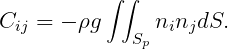 | (15.77) |
Except as noted below there are no other restoring coefficients.
If the configuration parameter ICCFSP=1 is assigned, additional ‘external’ restoring coefficients are included which represent the force on the body if there is a chamber of constant volume enclosing the pressure surface, with the assumption that compressibility effects are negligible. In this case the pressure in the chamber acts both on the water below and on the body above the chamber, to give additional forces and moments on the body. The only nonzero external restoring coefficients are
15.12 LOW-FREQUENCY LIMITS IN FINITE DEPTH OR IN A CHANNEL
If the depth H is finite and the frequency ω → 0, it follows from (15.5) that kH << 1 and KH = ω2H∕g = O(kH)2. In this case the far-field approximation of the Green function (15.18) is (cf [1], equation 10b)
![π [ ]
G (x;ξξξ) ≃ - ---[Y0(kR ) + iJ0(kR )] ≃ - (2∕H ) log (12kR ) + γ - iπ∕H
H](images/wamit_v74manual209x.png) | (15.79) |
Here J0 and Y 0 are the Bessel functions of order zero and R2 = (x - ξ)2 + (y - η)2. In the limit ω = 0 the Green function for a source between two horizontal rigid plates is used, where the corresponding far-field approximation is
 | (15.80) |
The difference between these two approximations is the complex constant
![[ 1 ]
c = - (2∕H ) log(2kH ) + γ - iπ∕H](images/wamit_v74manual211x.png) | (15.81) |
If the body is on the free surface, vertical (heaving) motion will cause a source-like flow in the far field proportional to the area of the waterplane, and similarly for roll and pitch motions if these are not cancelled by symmetry. Thus for any combination of modes (i,j) where the hydrostatic restoring coefficient Cij is nonzero, the pressure associated with the constant (15.81) will result in a difference between the added-mass and damping coefficients at low frequencies, relative to the computed limiting value for ω = 0. The asymptotic values of these coefficients for low frequencies are as follows:
 | (15.82) |
Here ij(0) is the value of the added-mass coefficient computed in the zero-frequency limit, the bars denote the nondimensional forms defined in Section 3.1 and Section 3.2, and the length scale L is defined by the input parameter ULEN in the GDF file. The mode indices (i,j) are restricted to the range (3-5) to include heave, roll and pitch.
Similar differences exist in a channel of finite width w, following the procedure in Section 12.7. In a channel of finite depth the complex constant analogous to (15.81) is
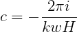 | (15.83) |
Thus
 | (15.84) |
If the channel depth is infinite
![c = - (4∕w )[log(Kw ) + γ + iπ ],](images/wamit_v74manual215x.png) | (15.85) |
and the last term in (15.82) affects both the added mass and damping.
15.13 FLUID DAMPING SURFACES
This section describes the equations used for damping surfaces in the fluid or on the free surface, following the procedure in Section 12.8. Two types of surfaces are considered: (a) submerged surfaces of zero thickness, represented by dipoles, and (b) surfaces on the free surface, referred to as ‘lids’. Several options are supported, based on the the parameter IDAMPER in the cfg file. If IDAMPER=-1 generalized modes are used to describe the deflection of the damping surfaces as in [Reference 31]. If IDAMPER=1, 2, or 3 the integral equations are modified to account for the damping surfaces without the need for generalized modes.
For dipole damping surfaces the pressure-jump across the surface is assumed to be proportional either to the normal velocity of the fluid (IDAMPER=1), with the boundary condition
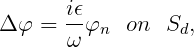 | (15.86) |
or to the relative normal velocity between the fluid and the normal velocity vn of the body at the same point (IDAMPER=2 or 3), with the boundary condition
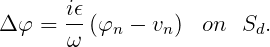 | (15.87) |
Here ϵ is the damping coefficient, represented by the parameter EDAMPER in the dmp file and in Section 12.8. It is convenient to write both boundary conditions in the common form
 | (15.88) |
where ψn = φn if IDAMPER=1, and ψn = φn - vn if IDAMPER>1.
Substituting (15.88) in (15.46) and (15.47) gives the following pair of integral equations for dipole dampers:
 | (15.89) |
if the field point x is on Sb, and
 | (15.90) |
if the field point x is on Sd. If IDAMPER=1 (15.89) and (15.90) are solved for the unknowns φ on Sb and φn = ψn on Sd. If IDAMPER=2 or 3 φn is replaced by ψn in the first term on the left-hand side of (15.90) and -4πvn is added on the right-hand side; then the two equations are solved for the unknowns φ on Sb and ψn on Sd. After solving for ψn on Sd, Δφ is evaluated from (15.88).
In the diffraction problem for the potential φD, the right-hand-side of (15.89) and (15.90) are replaced by 4πφ0(x) and 4πφ0n(x) as in (15.46) and (15.47). Since vn = 0 in this case φn = ψn on Sd, and the solution is the same for IDAMPER=1, 2 or 3. In the scattering problem, defined by (15.8), (15.89) and (15.90) are solved for the potential φS. In this case ψn = φDn and vn = -φ0n.
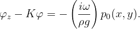
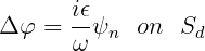
For damping lids on the free surface, the pressure is assumed proportional to the normal velocity. Thus
 | (15.91) |
and the free-surface condition (15.3) is replaced by
 | (15.92) |
The integral equation (15.11) is applicable, with the factor 4π used on the lid. Substituting φz for ni in (15.11) on Sd and using (15.92) gives the modified integral equation
 | (15.93) |
Here the fact that the Green function G satisfies the homogeneous free-surface condition is used in the integral over Sd. The factor 2π is used in the first term when x is on Sb and 4π is used when x is on Sd. In the diffraction problem for the potential φD, the right-hand-side of (15.93) is replaced by 4πφ0(x) as in (15.12).
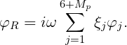
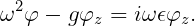
If IDAMPER=-1 the deflections of the damping surface Sd are represented by generalized modes, as in Chapter 9, and the analysis is similar to Reference [31]. If there are NEWMDS=N generalized modes, the total number of radiation modes for one body is J = N + 6, and the total potential is
 | (15.94) |
where
 | (15.95) |
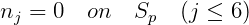
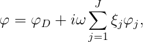
The body and damper are considered to be separate. Thus nj = 0 on Sd for j ≤ 6 and nj = 0 on Sb for j > 6. For dipole dampers, multiplying the boundary condition (15.86) by ni and integrating over Sd gives the equation
 | (15.96) |
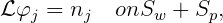
Similarly, using (15.92) for lid dampers,
 | (15.97) |
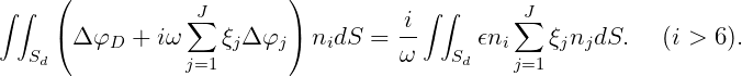
For i > 6 it follows from (15.96) and (15.97) that
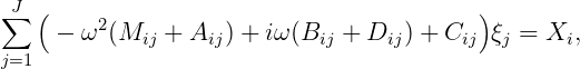 | (15.98) |
where
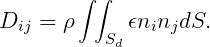 | (15.99) |
If i ≤ 6 or j ≤ 6 Dij = 0 and (15.98) is the same as the conventional equations of motion in Section 3.4. Thus (15.98) can be applied for all modes i. The coefficients Dij represent the damping effects and energy absorbed. The contribution from the real factor g∕ω2 on the right side of (15.97) is included in the hydrostatic coefficient Cij.