Chapter 3
DEFINITION OF QUANTITIES EVALUATED BY WAMIT
Cartesian coordinates are used to define the body geometry, forces, and other hydrodynamic quantities evaluated by WAMIT. These are output in nondimensional forms, in terms of the appropriate combinations of the water density ρ, the acceleration of gravity g, the incident-wave amplitude A, frequency ω, and the length scale L defined by the input parameter ULEN in the GDF file. The notation and definitions of physical quantities here correspond with those in Reference [3], except that in the latter reference the y axis is vertical.
The body geometry, motions and forces are defined in relation to the body coordinates (x,y,z), which can be different for each body if multiple bodies are analyzed. The z-axis must be vertical, and positive upwards. If planes of symmetry are defined for the body, the origin must be on these planes of symmetry. The global coordinates (X,Y,Z) are defined with Z = 0 in the plane of the undisturbed free surface, and the Z-axis positive upwards. The body coordinates for each body are related to the global coordinates by the array XBODY defined in Section 4.2.
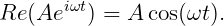
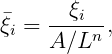
The incident-wave system is defined relative to the global coordinate system, and the phases of the exciting forces, motions, pressure and fluid velocity are defined relative to the incident-wave elevation at X = Y = 0. These outputs are defined in the general form
 | (3.1) |
where W = |U + iV | is the modulus and δ is the phase. With reference to equations (15.2) and (15.4), the incident-wave elevation at X = Y = 0 is equal to
 | (3.2) |
If δ > 0 the output leads the phase of the incident wave, and if δ < 0 the output lags the incident wave.
For field data (pressure, velocity, and free-surface elevation) and mean drift forces the definitions given below in Sections 3.5-3.8 apply to the complete solution for the combined radiation and diffraction problems. The components of the field data can be evaluated separately for either the radiation or diffraction problems using the configuration parameters INUMOPT5 and INUMOPT6, as explained in Sections 4.7 and 5.2.
For the sake of simplicity, the definitions which follow in this Section assume that the origin of the body coordinate system is located on the free surface. Special definitions apply to some quantities if vertical walls are defined, as explained in Section 12.4.
3.1 HYDROSTATIC DATA
All hydrostatic data can be expressed in the form of surface integrals over the mean body wetted surface Sb, by virtue of Gauss’ divergence theorem.
Volume:

All three forms of the volume are evaluated in WAMIT, as independent checks of the panel coordinates, and printed in the summary header of the output file where they are denoted by (VOLX, VOLY, VOLZ) respectively. The median volume of the three volumes is used for the internal computations. If it is less than 10-30, a warning is displayed and the coordinates of the center of buoyancy are set equal to zero. For bottom-mounted structures, where panels are not defined on the bottom, VOLZ differs from the correct submerged volume by the product of the bottom area and depth.
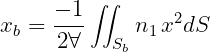
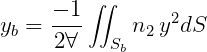
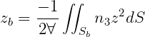
Coordinates of center of buoyancy:
Matrix of hydrostatic and gravitational restoring coefficients:
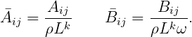
| C(3, 3) = ρg ∫ ∫ Sbn3dS | (3, 3) = C(3, 3)∕ρgL2 |
| C(3, 4) = ρg ∫ ∫ Sbyn3dS | (3, 4) = C(3, 4)∕ρgL3 |
| C(3, 5) = -ρg ∫ ∫ Sbxn3dS | (3, 5) = C(3, 5)∕ρgL3 |
| C(4, 4) = ρg ∫ ∫ Sby2n 3dS + ρg∀zb - mgzg | (4, 4) = C(4, 4)∕ρgL4 |
| C(4, 5) = -ρg ∫ ∫ Sbxyn3dS | (4, 5) = C(4, 5)∕ρgL4 |
| C(4, 6) = -ρg∀xb + mgxg | (4, 6) = C(4, 6)∕ρgL4 |
| C(5, 5) = ρg ∫ ∫ Sbx2n 3dS + ρg∀zb - mgzg | (5, 5) = C(5, 5)∕ρgL4 |
| C(5, 6) = -ρg∀yb + mgyg | (5, 6) = C(5, 6)∕ρgL4 |
where C(i,j) = C(j,i) for all i,j, except for C(4, 6) and C(5, 6). For all other values of the indices i,j, C(i,j) = 0. In particular, C(6, 4) = C(6, 5) = 0.
In C(4,4), C(4,6), C(5,5) and C(5,6), m denotes the body mass. When Alternative form 1 is used for the FRC file (Section 4.3) the body mass is computed from the relation m = ρ∀. When Alternative form 2 is used for the FRC file (Section 4.4) the body mass is defined by EXMASS(3,3).
3.2 ADDED-MASS AND DAMPING COEFFICIENTS
Here
3.3 EXCITING FORCES
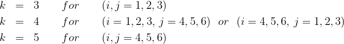
a) Exciting forces from the Haskind relations
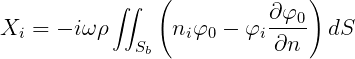
b) Exciting forces from direct integration of hydrodynamic pressure
where m = 2 for i = 1, 2, 3 and m = 3 for i = 4, 5, 6.
The separate Froude-Krylov and scattering components of the exciting forces can be evaluated, using the options IOPTN(2)=2 and IOPTN(3)=2 as described in Section 4.3. The Froude-Krylov component is defined as the contribution from the incident-wave potential φ0 and the scattering component is the remainder. Using the Haskind relations, these two components correspond respectively to the contributions from the first and second terms in parenthesis in the equation above. Using direct integration they correspond to the components of the total diffraction potential φD in equation 15.8.
3.4 BODY MOTIONS IN WAVES
Two alternative procedures are followed to evaluate the body motions in waves, corresponding respectively to the Alternative 1 (Section 4.3) and Alternative 2 (Section 4.4) FRC control files.
In Alternative 1, which is restricted to a body in free stable flotation without external constraints, the following relations hold


where m is the body mass and (xg,yg,zg) are the coordinates of the center of gravity.
The inertia matrix is defined as follows.
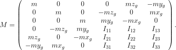 | (3.3) |
WAMIT equates the body mass to the mass of the displaced water in free flotation. The moments of inertia Iij are defined in terms of the corresponding radii of gyration rij, defined by the relation
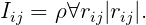
The array XPRDCT(I,J) input to WAMIT contains the radii of gyration input with the same units of length as the length scale ULEN defined in the panel data file.
In the Alternative 2 format of the FRC file the matrices Mij + MijE, B ijE and C ijE are input by the user to include the possibility of external force/moment constraints acting on the body.
The complex amplitudes of the body’s motions ξj are obtained from the solution of the 6×6 linear system, obtained by applying Newton’s law
![∑6 [ ]
- ω2 (Mij + M Eij + Aij) + iω(Bij + BEi,j) + (Cij + CEij) ξj = Xi.
j=1](images/wamit_v74manual16x.png)
where the matrices MijE, B ijE and C ijE are included only in the Alternative 2 case. Note that in the Alternative 2 case the user must specify the body inertia matrix Mij and include it in the total inertia matrix Mij + MijE specified in the FRC file.
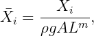
The non-dimensional definitions of the body motions are
where n = 0 for i = 1, 2, 3 and n = 1 for i = 4, 5, 6. The rotational motions (ξ4,ξ5,ξ6) are measured in radians.
3.5 HYDRODYNAMIC PRESSURE
The complex unsteady hydrodynamic pressure on the body boundary or in the fluid domain is related to the velocity potential by the linearized Bernoulli equation
The total velocity potential is defined by
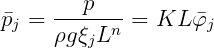
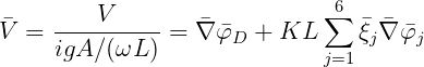
where the radiation and diffraction velocity potentials are defined in Section 15.1. The nondimensional velocity potential and hydrodynamic pressure are defined as follows:
where K = ω2∕g and
with n = 0 for j = 1, 2, 3 and n = 1 for j = 4, 5, 6.
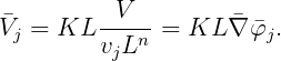
The body pressure can be evaluated separately for the diffraction or radiation problems by assigning the configuration parameters INUMOPT5=1 and/or INUMOPT6=1, as explained in Section 4.7. When the radiation components are output separately, the nondimensional pressure due to jth mode is defined by
Special definitions are required in the limits of zero and infinite wave periods, as explained in Section 3.9.
3.6 FREE-SURFACE ELEVATION
The free surface elevation is obtained from the dynamic free-surface condition
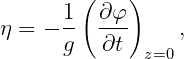
and in nondimensional form
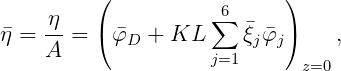
where is defined as in Section 3.5. (The nondimensional hydrodynamic pressure and wave elevation are equal to the nondimensional velocity potential at the respective positions.)
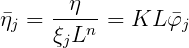
These parameters can be evaluated separately for the diffraction or radiation problems by assigning the configuration parameter INUMOPT6=1, as explained in Section 4.7. When the radiation components are output separately, the nondimensional free-surface elevation due to jth mode is defined by
The evaluation of the pressure or free-surface elevation requires special caution close to the body surface. Within a distance on the order of the dimensions of the adjacent panel(s), field-point quantities cannot be computed reliably. More specific limits can be ascertained by performing a sequence of computations and studying the continuity of the result. Approaching the body along a line normal to the centroid of a panel will minimize this problem. See Reference [12] regarding the computation of run-up at the intersection of the body and free surface. The parameter TOLFPTWL can be used to check for field points on the free surface which are close to, or inside, body waterlines (see Section 4.3).
3.7 VELOCITY VECTOR ON THE BODY AND IN THE FLUID DOMAIN
The nondimensional velocities evaluated by WAMIT are defined in vector form by
where

These parameters can be evaluated separately for the diffraction or radiation problems by assigning the configuration parameters INUMOPT5=1 and/or INUMOPT6=1, as explained in Section 4.7.
The evaluation of the velocity requires special caution close to the body surface, in the same manner as the pressure and free-surface elevation.
When the radiation components are output separately, the nondimensional velocity due to jth mode is defined by
Special definitions are required in the limits of zero and infinite wave periods, as explained in Section 3.9.
3.8 MEAN DRIFT FORCE AND MOMENT
The definition of the nondimensional mean drift force and moment in unidirectional waves is
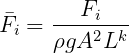
where k = 1 for the forces (i = 1, 2, 3), and k = 2 for the moments (i = 4, 5, 6).
For bi-directional waves of the same period, with complex amplitudes (A1, A2) and corresponding angles of incidence (β1, β2), the nondimensional outputs i(β1,β2) are the coefficients such that the total dimensional mean drift force or moment exerted on the body is given by the equation
![k 2 2 *
Fi(β1,β2) = ρgL (|A1 |Fi(β1,β1 ) + |A2| Fi(β2,β2) + 2Re [A1A 2Fi(β1,β2)]).](images/wamit_v74manual30x.png)
In Option 7 the drift force and moment are evaluated based on the momentum flux across a control surface as described in Chapter 11, using equations (15.57-60).
In Option 8, the evaluation of the horizontal drift force and vertical moment is based on the momentum conservation principle in its general form (see References [4] and [26]), without the assumption of energy conservation. This permits the analysis of cases where the body motions are affected by non-conservative effects, such as external damping. The azimuthal integration required to evaluate the momentum flux is performed by an adaptive quadrature formula. The integration is performed iteratively, with convergence specified by the criterion of absolute or relative errors in each drift force less than TOL=10-4. The maximum number of iterations is controlled by the parameter MAXMIT. A warning message is displayed in the event that this convergence criterion is not satisfied. See Section 5.8 for further information regarding the interpretation and control of this warning message.
Often the warning message is issued because the length scale parameter ULEN is much smaller than the relevant length scale of the body. Since the drift force increases in proportion to length, and the moment in proportion to (length)2, relatively small differences between large values may not be significant. In this case the warning message can be avoided by increasing ULEN to a value more representative of the length.
This force or moment can be either converged for most practical purposes or too small to be important in practice. It is recommended to check the practical importance of this quantity. Further check on the convergence of the result can be made by increasing MAXMIT gradually. Since the computational time increases exponentially, it is not recommended to use significantly large MAXMIT than the default value.
In Option 9, the evaluation of the drift force and moment is based on integration of the pressure over the body surface, using the relations in [10] and [17], as summarized in Section 15.7.
In Options 7 and 9, the mean drift force and moment evaluated from pressure integration and from momentum flux on a control surface are defined with respect to the body coordinate system. Conversely, the mean drift force and moment evaluated from momentum conservation in Option 8 are defined with respect to the global coordinate system.
3.9 ZERO AND INFINITE WAVE PERIODS
It is possible to evaluate the added mass (Option 1), and also the pressure and fluid velocity (Options 5 and 6) in the limiting cases of zero and infinite period (or equivalently, infinite and zero frequency), by inputting PER=0.0 and PER<0.0 in the POT file (see Section 4.2). This extension is particularly important in the context of evaluating the corresponding time-domain impulse response functions, as explained in Chapter 13.
The definition of the added-mass and damping coefficients is the same as shown in Section 3.2. Except as noted below, the damping coefficients are equal to zero in these limits. All other force coefficients are zero in these limits, with the exception of the heave exciting force and horizontal exciting moments, which tend to nonzero hydrostatic limits at zero frequency.
Special attention is required in the zero-frequency limit (ω = 0) if the fluid depth H is finite, or in a channel of finite width. Since the rigid-free-surface condition applies, the potential for rigid-body motions is non-unique within an arbitrary constant. For a body which is on the free surface this constant affects the added-mass and damping coefficients for heave, and also for the roll and pitch modes if these are coupled to heave due to non-symmetry. For these special cases the damping coefficients tend to non-zero limiting values as ω → 0, in a fluid of finite depth, and the added-mass coefficients are logarithmically infinite. In a channel of finite width the situation is somewhat different. Special formulae for evaluating these coefficients are given in Section 15.12.
In certain cases it is not possible to evaluate these limits. If the body surface includes horizontal panels or patches that are in the plane of the free surface (Z = 0) the infinite-frequency limit cannot be evaluated. Similarly, the zero-frequency limit cannot be evaluated if there is a free-surface pressure assigned on (Z = 0) (see Section 12.5). Neither of these limits can be evaluated if fluid dampers are used (see Section 12.8). If illegal wave periods are input in the pot file under these conditions, the run continues with a warning message stating that the period has been removed.
Special definitions are applied to the radiation pressure and velocity in the case of zero frequency (infinite wave period), which is identified in the output files by a negative value of the parameter PER, and also in the case of infinite frequency (zero wave period), which is identified by PER=0. In general, for nonzero finite values of the frequency, the nondimensional outputs for the radiation pressure and velocity are as defined in Sections 3.5 and 3.7. Thus the output pressure for each radiation mode is KLj and the output velocity for each mode is KLj. However for the two limiting cases, where KL = 0 or KL = ∞, the factor KL is omitted from the outputs for Options 5 and 6. The following table summarizes these definitions:
| frequency | period | pressure | velocity | |
| PER<0 | ω = 0 | ∞ | j | j |
| 0 <PER< ∞ | 0 < ω < ∞ | (2π∕ω) | KLj | KLj |
| PER=0 | ω = ∞ | 0 | j | j |
In order to output the radiation pressure and velocity for zero and infinite wave periods it is necessary to use the parameters INUMOPT5=1 and/or INUMOPT6=1 in the configuration file (see Section 4.7) or, alternatively, assign only one radiation mode in the potential control file and assign IOPTN(4)=0 in the force control file.