Chapter 14
COMPUTATIONAL TOPICS
In this Chapter various topics are covered which affect the use of WAMIT, especially for more advanced applications with complicated geometry, or multiple structures. These require a large number of panels in the low-order method, or corresponding number of unknowns in the higher-order method, to represent both the geometry and the hydrodynamic solution with a satisfactory degree of accuracy. In such cases the required storage for temporary data and the time required to set up and solve the linear systems of equations are both large.
From the computational standpoint the principal task is to set up and solve the linear systems of equations which correspond to the discretized integral equations described in Sections 15.3 and 15.5. The dimension of these linear systems is denoted by NEQN (number of equations). In the low-order method NEQN is the same as the number of panels. In the higher-order method NEQN depends on the number of patches, panels, and on the order of the basis functions, as explained in Section 14.1.
WAMIT includes three optional methods for solving the linear systems of equations, including a direct solver which is robust but time-consuming for large values of NEQN, an iterative solver which for large systems of equations is much faster, and a block-iterative solver which combines the advantages of each to some extent. These methods are described and compared in Section 14.2.
Section 14.3 describes the required storage for the influence coefficients on the left-hand-sides of the linear systems of equations. These must be stored either in random-access-memory (RAM) or in scratch files on the hard disk. Since access to RAM is much faster, this option is advantageous from the standpoint of computing time if sufficient RAM is available. Section 14.4 describes the procedure to allocate the data storage between RAM and the hard disk in an efficient manner. Section 14.5 explains details associated with the use of scratch files on the hard disk.
The advantages and use of multiple processors are described in Section 14.6, including a comparison of computing times for two applications. This shows the dramatic reduction in computing time that can be achieved when the number of CPUs is increased. However the use of multiple CPUs requires a proportionally large size of RAM.
Section 14.7 gives instructions for users to modify the WAMIT DLL files geomxact and newmodes. Section 14.8 lists the filenames which are reserved for use by WAMIT.
14.1 NUMBER OF EQUATIONS (NEQN) AND LEFT-HAND SIDES (NLHS)
In the low-order method (ILOWHI=0) the number of equations depends on the number of panels NPAN specified in the GDF input file(s). In the higher-order method (ILOWHI=1) NEQN depends on the number of patches, and on the spline paramters NU, NV, KU, and KV. NEQN is modified if the body geometry is reflected about planes of symmetry, automatic discretization of the interior free surface is utilized (IRR>1), or waterline trimming is used (ITRIMWL>0). The value of NEQN for each run is listed in the header of the .out output file. Typical values of NEQN are between 100 and 10,000. NEQN is always equal to the number of unknowns in the representation of the velocity potential on the body surface (and interior free surface if IRR≥1).
The body surface is defined in the .gdf file on NPAN panels in the low-order method or NPATCH patches in the higher-order method. the .gdf file also specifies the symmetry indices ISX,ISY, which define planes of symmetry (x = 0, y = 0 respectively) for the body as explained in Chapters 6 and 7. If one or two planes of symmetry are defined, only one half or one quarter of the body surface is defined in the .gdf file. The program uses these symmetries to reduce NEQN, when it is possible to do so, by defining separate solutions which are symmetric and antisymmetric with respect to each plane of symmetry. The number of the corresponding sets of influence functions, or left-hand sides, is denoted by NLHS. If there are no planes of symmetry NLHS=1, with one plane of symmetry NLHS=2, and with two planes of symmetry NLHS=4.
Before considering possible modifications which may be required, the value of NEQN is defined based on the inputs in the .gdf file. In the low-order method NEQN=NPAN is the number of panels on this surface. In the higher-order method
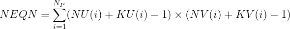 | (14.1) |
Here NP =NPATCH is the number of patches, NU and NV are the numbers of panels on each patch, and KU and KV are the orders of the B-splines used to represent the solution, as explained in Section 7.2.
If the irregular-frequency removal option is used with IRR=1, the interior free-surface is included as a part of the surface defined in the gdf file, and the value of NEQN defined above is unchanged. But if automatic discretization of the interior free surface is utilized (IRR>1) NEQN is increased by the program to include the additional unknowns on the interior free surface. (See Chapter 10.)
If waterline trimming is used (ITRIMWL=1) the value of NEQN may change, either increasing or decreasing depending on the trimming displacement and angles. (See Section 12.2.)
Reflection is performed automatically by the program if the planes of geometric symmetry (x = 0 and/or y = 0 of the body coordinate system) do not coincide with the X = 0 and/or Y = 0 planes of the global coordinate system. This may occur in the following cases:
- if the input parameters XBODY(1), XBODY(2), or XBODY(4) which define the origin of the body coordinate system are nonzero in the POT file (See Section 4.2)
- for bodies near vertical walls (Section 12.4)
- for multiple bodies (NBODY>1) as explained in Chapter 8
- If the trim angle about the x-axis is nonzero, symmetry about the plane y = 0 is destroyed, and vice-versa. In these cases the body surface is reflected, NEQN is increased, and NLHS is decreased.
When reflection about one plane of symmetry is required, NEQN is increased by a factor of two and NLHS is reduced by a factor of one-half. When reflections about two planes of symmetry are required, NEQN is increased by a factor of four and NLHS is reduced by a factor of one-quarter.
Flow symmetries and anti-symmetries are enforced in the solution of the integral equations by the method of images. The collocation point xi in the argument of the wave source potential, is reflected about the geometry symmetry planes with a factor of +1 or -1 for symmetric and antisymmetric flow, respectively.
Since the issue of hydrodynamic symmetry is so important, it should be emphasized that the separate analysis of symmetric and antisymmetric modes of motion applies not only to the obvious cases of radiation modes, such as surge, sway, and heave, but also to the more complex solution of the diffraction problem, even in oblique waves. This is achieved in WAMIT by decomposing the complete diffraction (or scattering) solution as the sum of four separate components that are respectively even or odd functions of the horizontal coordinates. Physically these can be interpreted as the solutions of problems where standing waves are incident upon the body.
To avoid unnecessary computations, the architecture of WAMIT permits the analysis of any desired sub-set of the rigid-body modes and of the corresponding diffraction components, based on the settings of the MODE(I) indices in the potential control file (see Section 4.2). For example, if only the heave mode is specified in conjunction with the solution of the diffraction problem, and if there are planes of symmetry, only the symmetric component of the diffraction potential is evaluated. For this reason it is necessary to specify the complete diffraction solution (IDIFF= 1) to evaluate field data (free surface elevation, pressure, and fluid velocity) or to evaluate the drift forces. A warning message is displayed in cases where the solution of the diffraction problem is incomplete.
14.2 SOLUTION OF THE LINEAR SYSTEMS
WAMIT includes three optional methods for solving the linear systems of equations, including a direct solver which is relatively robust but time-consuming, an iterative solver which for large systems of equations is much faster, and a block-iterative solver which combines the advantages of each to some extent. The parameter ISOLVE in the configuration file is used to select which method is used for the run.
With the default value ISOLVE=0, WAMIT solves the linear systems by means of a special iterative solver. The maximum number of iterations is controlled by the parameter MAXITT in the configuration files (See Section 4.7), with the default value equal to 35. If convergence is not archieved within this limit a warning message is issued, and the computation continues without interruption. If the number of iterations displayed in the output is equal to MAXITT, this also indicates that convergence does not occur. The time required for this method is proportional to (NEQN)2 times the number of iterations. For large NEQN this is much faster than the methods described below. Another advantage of the iterative solver is that it does not require temporary storage proportional to (NEQN)2.
The direct solver (ISOLVE=1) is useful for cases where the iterative solver does not converge, or requires a very large number of iterations to achieve convergence. The direct solver is based on standard Gauss reduction, with partial pivoting. The LUD algorithm is employed for efficiency in solving several linear systems simultaneously, with different right-hand sides. The time required for this method is proportional to (NEQN)3. In cases where NEQN is relatively small the direct solver can result in reduced computing time, particularly if the number of right-hand sides is large. The direct solver requires sufficient RAM to store at least one complete set of (NEQN)2 influence coefficients.
The block-iterative solver (ISOLVE≥2) provides increased options in the solution of the linear system. This solver is based on the same algorithm as the iterative solver, but local LU decompositions are performed for specified blocks adjacent to the main diagonal. Back substitution is performed for each block, at each stage of iteration. This accelerates the rate of convergence, and as the dimension of the blocks increases the limiting case is the same as the direct solver. The opposite limit is the case when the dimension of the blocks is one, which is the result of setting ISOLVE=NEQN; in this case the result is identical to using the iterative solver without blocks (ISOLVE=0).
The iterative method is useful primarily for the low–order method, where NEQN is relatively large and the rate of convergence is good in most cases. Usually in the low-order method the number of iterations required to obtain convergence is in the range 10-20. In the standard test runs described in Appendicies A using the low-order method, the iterative or block-iterative solvers converge within the default number of iterations MAXITT=35, for all cases except TEST01b.
Experience using the low-order method has shown that slow convergence is infrequent, and limited generally to special applications where there either is a hydrodynamic resonance in the fluid domain, as in the gap between two adjacent barges, or in the non-physical domain exterior to the fluid volume. An example of the latter is a barge of very shallow draft, where the irregular frequencies are associated with non-physical modes of resonant wave motion inside the barge. These types of problems can often be overcome by modifying the arrangement of the panels or increasing the number of panels.
For the higher-order method the linear system loses diagonal dominance as the order of the basis functions increases, as shown in the expression for dikH in (15.32). Experience indicates that the convergence rate is reduced, and it is generally advisable to use the direct solver (ISOLVE= 1) or, if necessary in cases where NEQN is very large, the block-iterative solver (ISOLVE> 1).
Results from convergence tests using the low-order method have been published in References 5, 6, 9, 10 and 12. The accuracy of the evaluated quantities has been found to increase with increasing numbers of panels, thus ensuring the convergence of the discretization scheme. The condition number of the linear systems is relatively insensitive to the order of the linear systems, and sufficiently small to permit the use of single-precision arithmetic. Convergence tests for the higher-order method are reported in References 18, 19, 20, 24 and 25.
14.3 TEMPORARY DATA STORAGE
From the computational standpoint the principal tasks are to set up and solve the linear systems of equations for the unknown potentials and source strengths. These tasks require substantial temporary storage for most practical applications, either in RAM (random-access memory) or in scratch files on the hard disk. Generally access to RAM is much faster than to the hard disk, but the size of RAM is relatively small. The first versions of WAMIT were developed when RAM was quite small (typically measured in Kilobytes) and it was essential to use scratch files whenever possible. WAMIT Version 7 has been developed to take advantage of the much larger RAM available in contemporary systems, measured in Gigabytes (1 GB is equal to 109 bytes or 106 Kilobytes).
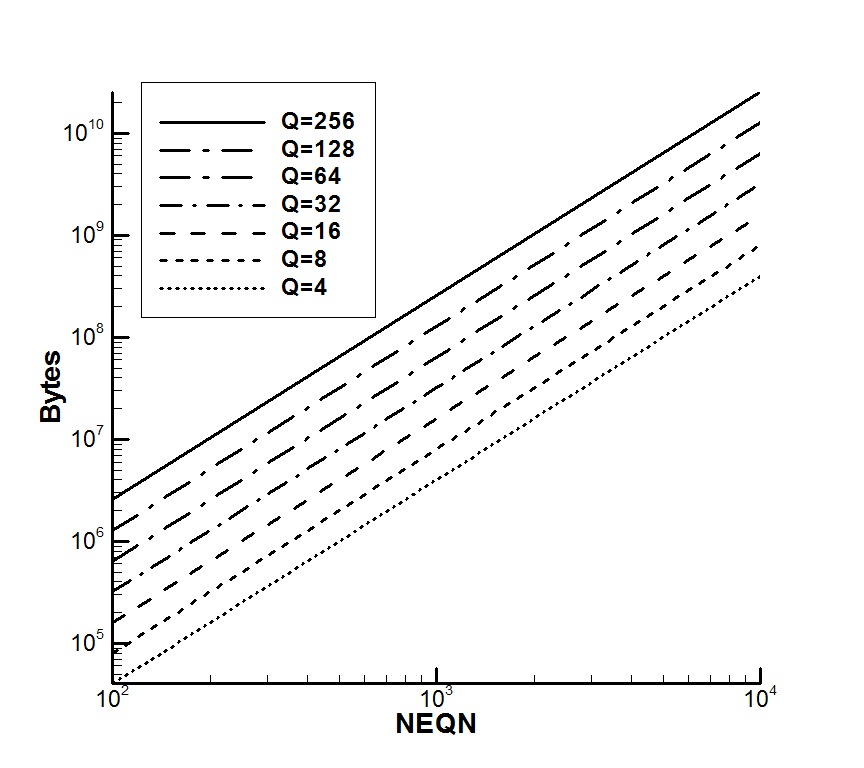
For most applications the dominant storage requirement is for the (NEQN)2 influence coefficients on the left-hand-side of the linear systems of equations. Since typical values of NEQN are between 100 and 10,000, between 104 and 108 influence coefficients must be stored for each left-hand-side. Here we consider only the storage of these matrices, since other data storage requirements are negligible by comparison.
The influence coefficients are related to the free-surface Green function and its derivatives, as defined in Section 15.2. These include real components associated with the Rankine source potential 1∕r, and complex components associated with the effect of the free surface (cf. Equations 15.14-18). To avoid redundant computations the real components are evaluated only once, whereas the complex components must be evaluated separately for each wave period. Thus separate storage is required for the real and complex matrices. The estimated storage for each of these is described below.
WAMIT takes into account flow symmetries in setting up the linear systems, to minimize NEQN. When planes of symmetry exist with respect to the planes X = 0 and/or Y = 0, NEQN can be reduced by one half in each case, thus reducing the number of influence coefficients on one left-hand side by a factor of 1/4 or 1/16. In general, the number of left-hand-sides NLHS must be increased by 2 or 4 in order to solve both the symmetric and anti-symmetric problems (e.g. heave and surge in the case of a body which is symmetric about X = 0). Depending on the number of relevant modes and symmetry planes, NLHS=1,2 or 4.
The minimum number of influence coefficients which must be stored is equal to the product NLHS×(NEQN)2. However additional matrices may be required, depending on the input parameters ILOG and ISOR in the configuration file. ILOG=0 or 1 in all cases. ISOR=0 or 1 for the low-order panel method, and ISOR=0 for the higher-order method. For the real components 4 bytes are required for each coefficient, and the total storage required for all matrices is Sr = Qr(NEQN)2 where
 | (14.2) |
For the complex components 8 bytes are required for each coefficient, and the total storage required for all matrices is Sc = Qc(NEQN)2 where
 | (14.3) |
These can be estimated using Figure 14.1, with the factor Q defined in (14.2-3). Note that 4 ≤ Qr ≤ 160 and 8 ≤ Qc ≤ 64. In three special cases Qr is greater by a relatively small amount: (1) in the low-order method if the scattering parameter ISCATT=1 in the configuration files, (2) if pressure surface panels or patches are used, as described in Section 12.5, or (3) if PER=0 is assigned in the POT file corresponding to zero wave period or infinite frequency. More significantly, if multiple processors are used (NCPU>1), the factor Qc must be multiplied by NCPU (See Section 14.6).
14.4 DATA STORAGE IN RAM
In Version 7 provisions have been made to replace scratch files on the hard disk by arrays in RAM, up to the limit of RAM that is available. This can save substantial computing time. To fully utilize this capability, the user should assign the parameter RAMGBMAX in the configuration file, as described in Section 4.7, based on the estimated amount of RAM that is not required for other purposes. Some experience may be required to determine this input. For a system that is not used concurrently for other substantial computations, a suggested estimate is one-half of the total RAM if the RAM is less than 2 Gb, or the total RAM minus 1 Gb for systems with more than 2 Gb. For systems running under Windows the total RAM is displayed by the Control Panel System option. It is important not to assign a value of RAMGBMAX that is too large, since this may result in ‘paging’ or transfer of data to virtual memory on the hard disk, which will slow down the computations.
The parameter RAMGBMAX is based on the available memory of the system, and is not dependent on the inputs to each run. Thus it is recommended to assign RAMGBMAX in the file config.wam and not in the configuration file runid.cfg associated with a particular run. If RAMGBMAX is not assigned in the configuration files the default value 0.5 is used. An estimate of the actual RAM used for each run is shown in the output file wamitlog.txt.
If RAMGBMAX is sufficiently large, all of the real and complex influence coefficients are stored in RAM. In this case the total RAM required is estimated from Figure 14.1 with Q = Qr + NCPU × Qc. If this is not possible, the program will distribute the data between RAM and the hard disk using the following order of priorities:
- real coefficients are stored on the hard disk, leaving all available RAM for the storage of complex coefficients
- if NLHS>1, some but not all left-hand-side arrays are stored in RAM and the remainder on the hard disk
- if the RAM can not store one complete complex left-hand-side array, a subset of the coefficients are stored in RAM and the remainder on the hard disk
If multiple processors are used (NCPU>1) all of the complex arrays must be in RAM. Thus the minimum RAM required for multiple processing is estimated from Figure 14.1 with Q = NCPU × Qc. If this is not possible, execution of the program terminates with an error message advising the user to increase RAMGBMAX or reduce NCPU.
If NCPU=1 the following minimum requirements apply for available RAM:
- if ISOLVE=1 (direct solver) or ILOWHI=1 (higher-order method), one complete complex left-hand-side must be stored in RAM
- if ISOLVE>1 (block-iterative solver) one complex left-hand-side must be stored in RAM with dimensions equal to the maximum block size
14.5 DATA STORAGE IN SCRATCH FILES
Two types of temporary scratch files are opened during execution of the subprogram POTEN. One group are opened formally using the FORTRAN scratch file convention, with filenames which are assigned by the compiler. The second group are opened with the temporary filenames SCRATCHA, SCRATCHB, ..., SCRATCHO. All of these files are deleted prior to the end of the run, but if execution is interrupted by the user (or by power interruption to the system) some or all of these scratch files may remain on the hard disk. In the latter case the user is advised to delete these files manually.
If the storage requirements of a run exceed the available disk space a system error will be encountered; in this event the user should either increase the available disk space or reduce the number of panels or solutions. The parameter SCRATCH_PATH can be used in the configuration files to distribute storage between two disks, as explained in Section 4.7.
14.6 MULTIPLE PROCESSORS (NCPU>1)
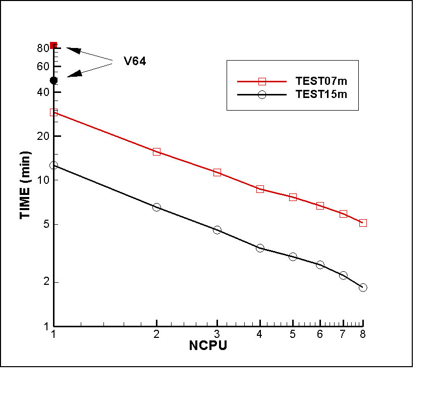
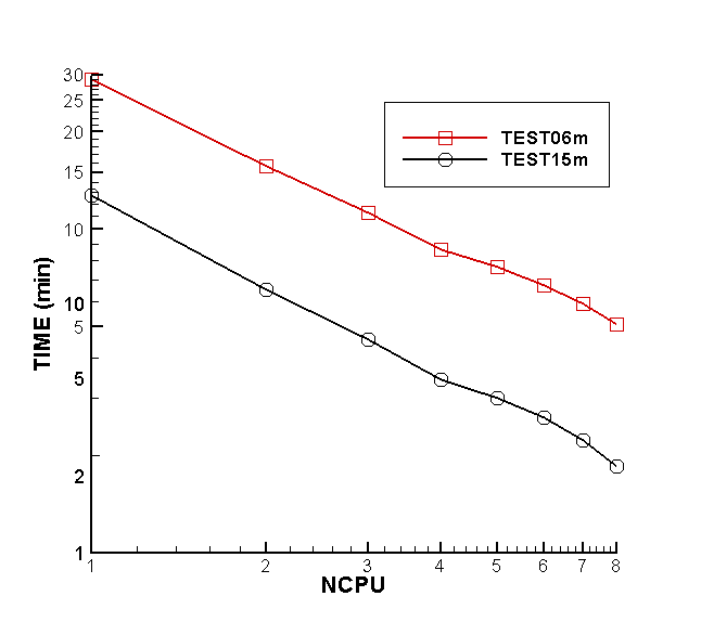
WAMIT Version 7.0pc is compiled with the Intel Fortran Compiler Version 12, using special directives to enable parallel processing on systems with multiple processors. Depending on the inputs and hardware, the total run time can be reduced substantially by using this capability. Figure 14.2 shows two examples, using modified inputs of the test runs 06a (ISSC TLP) and 15 (Semi-sub) which are described in Appendix A, and using the low-order and higher-order options respectively. In order to provide examples for relatively large computations, the input parameters for these two runs have been modified as explained in the caption.
Users should first verify the number of CPU’s and size of RAM of the system. (For Windows systems the RAM size is displayed after selecting ‘Start’, ‘Control Panel’, ‘System’. The number of processors is listed under ‘Advanced’, ‘Environment Variables’ ) NCPU should be determined based on the number of physical processors, also referred to as ‘cores’, and not based on the number of ‘hyper-threads’.
If the system includes more than one CPU, open the file config.wam with a text editor. The default settings in this file are as follows:
RAMGBMAX=0.5
Change NCPU to the appropriate number for the system, and increase RAMGBMAX to the maximum value which can be used for scratch memory, following the guidelines in Section 14.4. Note that the RAM required for multiple processing is proportional to NCPU. The actual RAM required during a run is displayed in the output file wamitlog.txt. If RAMGBMAX is not sufficiently large for the value of NCPU specified, the program stops with an error message displayed. In that case the user should reduce NCPU, or modify the other input parameters to increase RAMGBMAX or reduce the required RAM.
The principal advantage of multiple processing is in the computing time for loops over the wave period. During the run, when the time and number of iterations are output for each wave period on the monitor, these are displayed in groups of NCPU lines more-or-less simultaneously, with values of the wave period which usually are not in a logical sequence. (The original sequence is restored in the header of the .out output file, where it will be noted that the clock time for each wave period is not sequential.) Test14a is a useful example of this process, and of the advantage of using multiple processors for runs with a large number of wave periods (See Appendix A.14).
When NCPU>1, the value of NCPU used is shown in the wamitlog.txt output file. If the total number of wave periods NPER is less than the value of NCPU in the configuration files, NCPU is reduced for the loops over the wave period and the reduced value is displayed in the wamitlog.txt file. Maximum efficiency of the computing time is achieved when NPER is an integer multiple of NCPU.
When NCPU>1 the ‘BREAK’ option to interrupt the run is disabled and cannot be used (See Section 4.12).
14.7 MODIFYING DLL FILES
The files geomxact.f and newmodes.f can be modified by users following the instructions in Sections 7.9 and 9.3. This makes it possible for users to develop special subroutines for the definitions of the body geometry and generalized modes, respectively, and to link these subroutines with WAMIT at runtime.
WAMIT Version 7 is compiled with Intel Visual Fortran (Version 12.1). The previous Version 6.4PC was compiled with Intel Visual Fortran (Version 10.1) and earlier versions were compiled with Compaq Visual Fortran. Any of these Fortran compilers can be used to compile modified versions of the files geomxact.dll and newmodes.dll for use with a single processor (NCPU=1), using the following procedure:
- Open a new project ‘geomxact’ as a Fortran Dynamic Link Library
- Add geomxact.f to the project
- Build a release version of geomxact.dll
- Copy the new version of geomxact.dll to the working directory for WAMIT
The same procedure is used for NEWMODES, except for the different filenames.
Users who modify the DLL files for runs with multiple processors (NCPU>1) are advised to contact WAMIT Inc. for special instructions.
It may be possible to use other FORTRAN compilers to build the DLL files, but certain conventions in calling subroutines must be consistent with those of Intel Visual Fortran. Further information is provided in [23], Chapters 8 and 18.
14.8 RESERVED FILE NAMES
To avoid conflicting filenames, users are advised to reserve the extensions gdf, pot, frc, spl, p2f, out, pnl, fpt, pre, mod, hst, csf, csp, bpi, bpo, idf, rao, dmp, 1, 2, 3, 4, 5p, 5vx, 5vy, 5vz, 6p, 6vx, 6vy, 6vz, 7, 8,and 9 for WAMIT input and output. Other reserved filenames are config.wam, fnames.wam, break.wam, errorp.log, errorf.log, wamitlog.txt, SCRATCH* (where *=A,B,C,...,O), as well as wamit.exe, defmod.f, defmod.exe, the DLL files geomxact.dll and newmodes.dll, and the Intel DLL files listed in Section 2.1 which are required to execute the program. The utility f2t.exe described in Chapter 13 uses the reserved file inputs.f2t.
14.9 LARGE ARRAYS OF FIELD POINTS
Starting in WAMIT Version 7.1 there are two alternative options (NFIELD_LARGE=0 and NFIELD_LARGE=1) to evaluate the pressure and velocity at field points (FORCE Option 6).
In the default case, specified by the configuration parameter NFIELD_LARGE=0, these outputs are computed in the main loop over all wave periods together with all of the other outputs. (This is the same procedure as in all previous versions of WAMIT.) This procedure is efficient in most cases, especially if multiple-processing is used (NCPU>1) and the number of wave periods NPER is large. The computing time is minimized by pre-computing the Rankine components of the influence functions, which are independent of the wave period, for all combinations of field points and integration points on the body surface. If NFIELD is the number of field points and NBODYSURF is the number of integration points on the body, this requires the temporary storage of order NFIELD×NBODYSURF influence functions.
If NFIELD_LARGE=1 is specified in the configuration file, the evaluation of the field outputs is skipped in the period loop, and performed in a different order after the period loop is completed. In this case the loop is over the NFIELD field points, and the influence functions are computed within this loop. Thus the storage requirement is much smaller. If NCPU>1 the loop is parallelized. This alternative is most efficient if NFIELD is large, especially if NPER<NCPU.
The best choice between these two options will depend not only on the input parameters, but also on the computing system including the number of processors (NCPU) and size of RAM.