Wamit, Inc. - The State of the Art in Wave Interaction Analysis

Chapter 9
GENERALIZED BODY MODES (NEWMDS>0)

WAMIT includes the capability to analyze generalized modes of body motion, which extend beyond the normal six degrees of rigid-body translation and rotation. These generalized modes can be defined by the user to describe structural deformations, motions of hinged bodies, and a variety of other modes of motion which can be represented by specified distributions of normal velocity on the body surface. To simplify the discussion it will be assumed that only one body is analyzed, i.e. NBODY=1. The analysis of multiple bodies with generalized modes is discussed below in Section 9.5.

Each generalized mode is defined by specifying the normal velocity in the form
$φjn = nj = ujnx + vjny + wjnz$ (9.1)

where j > 6 is the index of the mode. (The first six indices j = 1, 2,..., 6 are reserved for the conventional rigid-body modes.) The displacement vector (u_j,v_j,w_j) is defined by the user in a special subroutine which can be accessed and modified by the user. The displacement vector can be any physically relevant real function of the body coordinates (x,y,z) which can be defined by FORTRAN code.

Corresponding to these modes are the generalized hydrodynamic force components, which are defined as in Sections 3.2 and 3.3 with the extended normal-vector n_i and the corresponding radiation solutions φ_i. Further discussion of the pertinent theory may be found in References [13] and [26].

The following examples are intended to illustrate applications. (The first four are simplified from the computational examples in [13].)

A ship with simplified transverse and vertical bending modes described by the Legendre polynomial of order 2:
$u = 0, v = P (q), w = 0 7 7 2 7$ (9.2)

$u8 = 0, v8 = 0, w8 = P2 (q)$ (9.3)

Here NEWMDS=2, P₂(q) = 3 2q² - 1 2 is the Legendre polynomial and q = 2x∕L is the normalized horizontal coordinate varying from -1 to +1 over the length L of the ship.
A vertical column, bottom mounted, with three orthogonal cantilever modes described by shifted Jacobi polynomials:
$2 u7 = q , v7 = 0, w7 = 0$ (9.4)

$3 2 u8 = 6q - 5q , v8 = 0, w8 = 0$ (9.5)

$u9 = 28q4 - 42q3 + 15q2, v9 = 0, w9 = 0$ (9.6)

Here NEWMDS=3, and (q = z∕HBOT + 1) is the normalized vertical coordinate varying from 0 at the bottom to 1 at the free surface.
Two bodies connected by a simple hinge joint at the origin, permitting each body to pitch independently about the y-axis. In this case the six rigid-body modes are defined as if the hinge is rigid, and the new mode (j = 7) is specified by the vector
$u = zn sgn (x), v = 0, w = |x |n 7 x 7 7 z$ (9.7)

with NEWMDS=1. Here sgn(x) is equal to 1 according as x > 0 or x < 0. Test 24, described in Appendix A.24, is a more complicated example with multiple hinges.
An array of five identical bodies, all described by panels in the same GDF file as if for a single body with five separate elements; the bodies are centered at transverse positions y = -4w,-2w, 0, 2w, 4w to simulate images of the central body in the presence of tank walls at y = w. The surge, heave, and pitch exciting forces on the central body are then specified by the exciting force coefficients X₇, X₈, X₉. The corresponding new modes are defined which have the same normal velocities on the central body and zero on the images. Here NEWMDS=3, and the vectors (u_j,v_j,w_j) are all zero, except in the range -w < y < w where
$u7 = 1$ (9.8)

$w = 1 8$ (9.9)

$u9 = z w9 = - x$ (9.10)

(With these definitions the exciting force coefficients can be evaluated either from the Haskind relations or direct pressure integrals as defined in Section 3.3, with the surface integrals extended over the ensemble of the central body and its images.)
A ship with a discontinuous shearing mode at the midship section, which can be used in conjunction with the fixed mode option (described in Section 4.5) to evaluate the shear force acting on the hull.

In cases such as examples 3 and 5 above where the modes are discontinuous, it is important when the higher-order method is used (ILOWHI=1) for the mode discontinuities to coincide with the boundaries between patches and not to occur within the interior of patches, as explained in Section 7.1.

In the generalized mode analysis one or two planes of geometric symmetry can be exploited to reduce the computational burden, when the body geometry permits. In such cases it is necessary to define the generalized modes to be either symmetrical or antisymmetrical. These symmetries must be specified in the subroutine by assigning one of the integers (1-6) to the array ISYM for each of the generalized modes. The value of this integer signifies that the symmetries of the generalized mode are the same as the corresponding rigid-body mode. Since the symmetries of surge (j=1) and pitch (j=5) are always the same, and likewise for sway (j=2) and roll (j=4), specifying ISYM=1 or 5 is equivalent, and similarly ISYM=2 or 4 is equivalent. If there are no planes of symmetry, any integer in the range (1-6) may be assigned to ISYM.

Any problem which can be analyzed with the NBODY option can also be analyzed with the generalized mode option. If geometric symmetry planes exist for the ensemble of all bodies, the use of the generalized mode method is more efficient computationally. On the other hand, the preparation of input files generally is simpler in the NBODY approach.

Complex generalized modes can be analyzed by superposition of the separate real and imaginary parts, each of which is treated as a separate real mode. For example, the specifications w₇ = cos(kx), w₈ = sin(kx) define two vertical deflections which can be superposed with a phase difference of 90^∘ to represent a snake-like traveling wave along the body.

Two alternative program units have been provided in the WAMIT software package to facilitate the use of generalized modes. The first method, also used with previous versions of WAMIT, uses a separate program DEFMOD to evaluate the geometric data associated with generalized modes. DEFMOD contains a subroutine DEFINE, which can be modified by the user to compute the displacement vector for different generalized modes. This method can only be used with the low-order method (ILOWHI=0). The second method, which is applicable for both the low-order and higher-order methods, uses a DLL file containing a special subroutine NEWMODES with a library of lower-level routines where different types of generalized modes can be defined. Since NEWMODES is contained in a DLL file it can be modified by the user, in a similar manner to the GEOMXACT file for defining bodies analytically (cf. Section 7.9).

The first method, using the program DEFMOD, can be used with any suitable FORTRAN compiler. Three separate runs must be made, first with WAMIT to set up the input file for DEFMOD, then with DEFMOD, and finally with WAMIT to solve for the potentials in the usual manner. In the second method only one run of WAMIT is required, however users of the PC executable code must compile the DLL file following the instructions below.

In Section 9.1 the input files are described for performing the generalized mode analysis for a single body. Section 9.2 describes the use of DEFMOD, and Section 9.3 describes the alternative use of the DLL file NEWMODES. The definitions of hydrostatic restoring coefficients are described in Section 9.4 and the analysis of multiple bodies (NBODY>1) is described in Section 9.5.

Several test runs are used to illustrate the use of generalized modes, including the use of both DEFMOD and NEWMODES and the appropriate input files. TEST08 (ILOWHI=0) and TEST18 (ILOWHI=1) analyze a bottom-mounted column with bending modes. TEST16 analyzes a rectangular barge with bending modes. TEST17(a,b) illustrates the use of generalized modes to analyze damped motions of a moonpool. TEST23 uses generalized modes to analyse a bank of ‘paddle’ wavemakers. TEST24 analyses the motions of a vessel with five separate segments connected by hinges. Further information is contained in the Appendix.

9.1 INPUT FILES

Two input parameters NEWMDS and IGENMDS control the implementation of the generalized mode option. NEWMDS specifies the number of generalized modes, with the default value zero. IGENMDS is an integer used to specify the definition of the generalized modes, using either the DEFMOD program or the NEWMODES subroutine library. IGENMDS is input in the configuration file. The default value IGENMDS=0 is used if the program DEFMOD is used, as explained in Section 9.2. If IGENMDS is nonzero, the DLL file NEWMODES is used. In the latter case, the value of IGENMDS can be used to identify appropriate subroutines within the NEWMODES library, as explained in Section 9.3.

Different values of IGENMDS may be assigned for each body if NBODY>1, and the body numbers must be included as shown in Section 8.4.

The definition of nondimensional outputs corresponding to each mode of motion cannot be specified in general, without prescribing the dimensions of each mode. To avoid this complication, the parameter ULEN should be set equal to 1.0 in the GDF file whenever generalized modes are analyzed. Except for this restriction, the GDF and POT input files are not changed.

In the POT file the six rigid-body modes can be specified as free or fixed in the usual manner, by appropriate choices of the index IRAD and array MODE (see Section 4.2). The program assumes that all generalized modes (j > 6) are free, and sets the array elements MODE(j) equal to one for these modes during the computations.

The options in FORCE have the same effect for generalized modes as for the rigid-body modes, except for restrictions on the mean drift forces evaluated by direct pressure integration (Option 9) and control surfaces (Option 7). The two horizontal drift forces and the vertical drift moment can be evaluated, including all pertinent motions of the body in the rigid-body and generalized modes, using the momentum analysis (Option 8). Options 9 and 7 cannot be used for bodies with generalized modes. In the analysis of multiple bodies (NBODY>1), where some but not all of the bodies have generalized modes, Options 9 and 7 can be used for the bodies with no generalized modes.

The Alternative Form 2 of the FRC file (IALTFRC=2) should be used to specify the appropriate mass, damping, and stiffness matrices for the body including its extended modes. For example, in case 1 above, to account for the mass and stiffness of the ship hull it is necessary to include corresponding 8 × 8 matrices which correctly specify these coefficients for the distribution of internal mass within the ship and for its bending motion.

Figure 9.1: Flow chart showing the use of WAMIT and DEFMOD to define and analyze generalized modes in the low-order method (ILOWHI=0). The number of generalized modes NEWMDS is specified in the configuration file. On the first run of WAMIT the centroid coordinates, area, normal vector n, and cross-product x×n are output for each panel to the file gdf.PRE, for pre-processing by the program DEFMOD. After modification by the user to specify the desired modes, DEFMOD is run with the input file gdf.PRE, to produce the output file gdf.MOD containing the normal velocity of each new mode at the panel centroids, and also the hydrostatic coefficients. After this pre-processing is completed, WAMIT is run again in the normal manner, as in the flow chart of Figure 1.1. Note that WAMIT reads the GDF and POT input files on both runs, although the data in the POT file is only used on the second run.

9.2 USING DEFMOD WITH THE LOW-ORDER METHOD

To facilitate the definition of the vectors (u_j,v_j,w_j) by users, a pre-processor program DEFMOD is provided in Fortran source code to input the values of the normal velocity for each generalized mode, at the centroid of each body panel. DEFMOD includes a short subroutine DEFINE, which can be modified by the user for each application. In the DEFMOD subroutine as provided, DEFINE evaluates the bending modes of the vertical column used in TEST08. (The same subroutine is included in NEWMODES and used for TEST18.) The four examples itemized in the introduction of this Chapter are included in separate files DEFINE.1, DEFINE.2, DEFINE.3, and DEFINE.4 to illustrate the preparation of appropriate subroutines. (Additional modes are included in these files.)

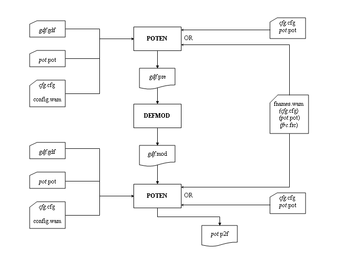
The evaluation of the normal velocity (9.1) for generalized modes requires a specification of the vectors u,v,w, and normal components n_x,n_y,n_z at the centroid of each panel. The first WAMIT run is aborted after writing these data to a file, and also the panel areas which are required to evaluate the hydrostatic coefficients for the generalized modes. The user is then requested to run DEFMOD. After DEFMOD is run, WAMIT may then be re-run to complete the analysis in the normal manner. This procedure is described in greater detail below, and illustrated by the flow chart in Figure 9.1. There are two input/output files associated with DEFMOD, both denoted by the filename (gdf) of the GDF file. The file gdf.PRE (for PRE-processing) contains for each panel the centroid coordinates x, the area, and the six components of n and x × n. The file gdf.MOD (for MODes) contains the generalized normal velocity on each panel, and the hydrostatic coefficients. These two files are prepared automatically by WAMIT and DEFMOD, and do not require special attention by the user.

The first run of WAMIT is made with NEWMDS > 0 specified in the configuration file. The pre-processor file gdf.PRE is output to the hard disk, and execution of WAMIT is interrupted with the following message:

‘PREMOD run completed – now run DEFMOD’

This first run of WAMIT is interrupted if NEWMDS > 0 and if there is not already in the default directory an input file with the name gdf.MOD. For this reason the user must rename or delete old MOD files prepared with the same gdf filename.

The output file gdf.PRE includes a one-line header for identification, followed by one line containing the symmetry indices (ISX, ISY), number of input panels (NEQN), and the maximum number of degrees of freedom which can be assigned in the WAMIT run (MAXDFR). Each of the remaining lines of this file corresponds to a panel, in the same order as the GDF file, and includes the coordinates x=(x,y,z) of the panel centroid, its area, and the six components of the normal vector n and cross-product x×n.

Either before or after the first run of WAMIT the user should modify the subroutine DEFINE in the program DEFMOD, specifying the number of generalized modes, their symmetries with respect to the geometric planes of symmetry of the body, and appropriate code for computing the vectors (u_j,v_j,w_j). DEFMOD should then be compiled and linked with an appropriate FORTRAN compiler. (Since DEFMOD is a self-contained FORTRAN file, linking is a trivial operation.)

DEFMOD is executed after the first run of WAMIT, using the gdf.PRE file as input to generate the output file gdf.MOD. This MOD file generated by DEFMOD includes the normal velocities of each generalized mode at each panel centroid. Also included at the end of this file are the generalized hydrostatic coefficients computed from equation (9.12).

After creating the gdf.MOD input file, execute WAMIT again to continue the run. From this on to the completion of the run the procedure is identical to that where NEWMDS=0.

The first and second runs are distinguished by the absence or presence, respectively, of the file gdf.MOD. Thus the existence of an old file with the same name is important. If changes are made only in the POT file (e.g. changing the wave periods), an existing MOD file can be reused without repeating the first run of WAMIT. On the other hand, if changes are made in the GDF file (e.g. changing the number of panels), and if the same gdf filename is used for the new GDF file, the old MOD file must be renamed or deleted before running WAMIT. If changes are made in DEFMOD (e.g. changing the definitions and/or number of new modes), the old PRE file can be used as input to create the new MOD file. A warning message is issued by DEFMOD before overwriting an old MOD file with the same name. No warning message is issued by WAMIT before overwriting an old PRE file with the same name.

9.3 USING THE DLL SUBROUTINE NEWMODES

The source code for the DLL file NEWMODES.F is provided with the WAMIT software to facilitate the specification of generalized modes by users. Users can compile their modified versions of NEWMODES, following the instructions below. This procedure is analogous to the modification of the DLL file GEOMXACT, as described in Section 7.9.

The file NEWMODES.F includes the main subroutine NEWMODES, and a library of specific subroutines used for different applications. The library can be modified or extended by users to describe generalized modes for other applications. In all cases the calls to these specific subroutines are made from NEWMODES. Thus the user has the capability to make appropriate modifications or extensions and to implement these with the executable version of WAMIT.

The principal inputs to NEWMODES are the Cartesian coordinates (X,Y,Z) of a point on the body surface, specified in the vector form X(1),X(2),X(3), and the corresponding components of the unit normal vector XN at the same point. These inputs are provided by the calling unit of WAMIT, and the user does not need to be concerned with providing these inputs. The principal outputs, which the user must specify for each generalized mode in an appropriate subroutine, are (1) the symmetry index of the mode, (2) the normal component of the displacement, and (3) the vertical component of the displacement. The symmetry indices, which are defined above in the Introduction, identify the symmetry of each mode (assuming the body has one or two planes of symmetry) by assigning the values (1,2,3,...,6) to indicate the same symmetries as the corresponding rigid-body modes. (Note that (sway/roll) and (surge/pitch) have the same symmetries. Thus the symmetry indices (2/4) and (1/5) are redundant, and either value can be assigned.)

The normal component of the displacement, denoted VELH in NEWMODES, is computed from the product of the displacement vector (U,V,W) and the normal vector XN. The vertical component of the displacement, denoted ZDISP in NEWMODES, is identical to the component W of the displacement vector (U,V,W).

Several other inputs are included in the argument list of NEWMODES to simplify its use and increase its computational efficiency. These include the body index IBI, the vector IBMOD which specifies the starting index for each body in the global array of mode indices, the patch/panel index IPP, the vector NEWMDS which specifies the number of generalized modes for each body, the integer IGENMDS specified in the configuration file, and an integer IFLAG which specifies the required outputs from each call. The inputs are explained in more detail below. Unit numbers for three files are also included in the argument list to facilitate input of user-defined data, and the output of error messages.

The body index IBI is useful for multiple-body computations, where different generalized modes may be specified on each body. If NBODY=1, the index IBI=1.

For the analysis of a single body, the mode index j is assigned consecutively as explained after equation (9.1), with the first generalized mode j = 7 and the last generalized mode j = 6 + NEWMDS(1). For multiple bodies the arrays for each body are concatenated in succession. The vector IBMOD(1:NBODY) points to the last mode index j used for the preceding body. Thus, in general, for body IBI, the first generalized mode is j = IBMOD(IBI) + 7 and the last generalized mode is j = IBMOD(IBI) + 6 + NEWMDS(IBI). Thus the pointer IBMOD is useful to assign generalized modes correctly when multiple bodies are analyzed.

The patch/panel index IPP can be used to identify specific portions of the body. IPP is the local panel or patch number of the body, as listed in the corresponding GDF file.

When NEWMODES is used to define generalized modes, the input IGENMDS must be specified in the configuration files with a nonzero value. Different values of IGENMDS can be useful in NEWMODES to identify different subroutines of the library. This is illustrated in the version supplied with WAMIT, where the integers 16, 17, 18 are used to identify the corresponding test runs and associated subroutines.

The input IFLAG is generated internally by the calling routine, with three possible values. Initially NEWMODES is called once with IFLAG=-1, to assign the array IMODE specifying the symmetry index for each mode. In subsequent calls where only the normal component of the displacement vector VELH is required, IFLAG=1. If both VELH and the vertical component ZDISP are required (for computations of hydrostatic coefficients) IFLAG=2. In the higher-order method a large number of calls are made to NEWMODES with IFLAG=1. If computational efficiency is important this should be considered in modifying or extending the subroutines in NEWMODES.

The comments inserted in the NEWMODES file should be consulted for further details.

Regardless if NEWMODES is used or not, the file newmodes.dll must be in the same directory as WAMIT.EXE.

Instructions for making new DLL files are included in Section 14.7.

In some cases it is useful to input data from a special input file, so that the subroutines in NEWMODES can be used with different values of relevant parameters. The following arguments have been added to NEWMODES to facilitate this procedure:

IFILEDLL is the unit number assigned by WAMIT to open and read the special data file. This unit number should be used in all cases so that there is no conflict with other files used by WAMIT for input and output.

FILENDLL is the filename gdf of the GDF input file gdf.GDF for the same body. This may be used optionally to distinguish between different special input data files. Examples are explained below for TEST23 and TEST24.

IERROR is the unit number assigned by WAMIT for the log files ERRORP.LOG and ERRORF.LOG, which are described in Section 10.1. Error messages which are generated in DLL subroutines can be added to the error files ERRORP.LOG and ERRORF.LOG by using the file number IERROR.

IWAMLOG is the unit number assigned by WAMIT for the log file WAMITLOG.TXT. This unit number can be used to copy the special input data file to the log file, as is done for other input files by WAMIT.

The use of this procedure, with a special input data file, is illustrated in TEST16, TEST18, TEST23 and TEST24. In TEST16 the subroutine FREEBEAM_X is used to represent the bending modes and the length of the beam is input from the special file test16_Length.dat. In TEST18 the subroutine JACOBI is used to represent the cantilever bending modes with shifted Jacobi polynomials, and the depth of the column is input from the special file test18_depth.dat. In TEST23 the subroutine WAVEMAKER inputs the depth of the hinge axis from a special file test23_wmkrhinge.dat. In TEST24 the subroutine HINGE_MODES inputs data from the file test24_xhinge.dat. Users who modify the DLL subroutines or make new DLL subroutines can follow the code in these subroutines for guidance in inputting data from an external file.

9.4 HYDROSTATICS

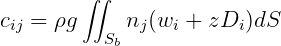
To evaluate the motions of a body including generalized modes, it is necessary to evaluate the corresponding hydrostatic coefficients. In general these are defined by the matrix (Reference 13, equation 2.17)
$∫∫ c = ρg n (w + zD )dS ij Sb j i i$ (9.11)

Here D_i denotes the divergence of the vector (u_i,v_i,w_i), assumed to be continuous in the vicinity of the body surface.

In cases where D_i = 0 the hydrostatic matrix can be evaluated uniquely from the vertical component w_i. For these cases the simplified hydrostatic matrix
$∫∫ cij = ρg njwidS Sb$ (9.12)

is computed and no further steps are required by the user. This computation is performed in DEFMOD if that program is used, or internally in WAMIT if the DLL subroutine NEWMODES is used.

In special applications where D_i≠0, the hydrostatic coefficients can be programmed specially by modifying the code in the main program of DEFMOD. Alternatively, the extra contribution from the last term in (9.11) can be included as an ‘external’ force, in the stiffness matrix of the FRC file.

The hydrostatic coefficients c_ij are output, as part of the complete hydrostatic matrix, in the file out.hst, with the format indicated in Section 5.6. (Here out denotes the filename of the .out file for the run.)

Note that the hydrostatic coefficients associated with generalized modes do not include gravitational restoring due to the internal mass of the body. Nonzero restoring effects due to gravity should be included as ’external’ force components in the stiffness matrix of the FRC file. The coupling between the generalized modes, and between the generalized and rigid-body modes, should be included. The gravitational force and moment associated with the rigid-body modes (i,j ≤ 6) should not be included since these components are evaluated in the program.

It is not possible for the program to evaluate the hydrostatic matrix in a unique manner which applies to all possible situations, including the effects of the gravitational force associated with the internal mass of the body. The coefficients evaluated and used by the program are specifically those defined by the matrix of hydrostatic and gravitational restoring coefficients listed in Section 3.1 for the rigid-body modes and by the hydrostatic matrix (9.12) for the generalized modes. Users should input additional restoring coefficients as necessary using the EXSTIF matrix.

9.5 NBODY ANALYSIS

The NBODY and generalized mode analyzes can be combined. An example where this might be effective is if two separate bodies are in close proximity, one or both of them are undergoing structural deflections, and there are no planes of geometric symmetry for the ensemble of two bodies.

If NBODY>1, separate values of NEWMDS and IGENMDS must be specified for each body. Both parameters are defined in the configuration file using separate lines for each body with the syntax ‘NEWMDS(m) = n’ ‘IGENMDS(m) = i’. Here m is the body index, n is the number of new modes for that body, and i is the value of IGENMDS appropriate for the same body. For example, if there are three bodies, and body 1 has 3 free beam bending modes defined by NEWMODES.DLL, body 2 has no generalized modes, and body 3 has 2 moonpool free-surface lids, four lines should be added to the configuration file as follows:

NEWMDS(1)=3
IGENMDS(1)=16
NEWMDS(3)=2
IGENMDS(3)=17

(It is not necessary to include the additional lines NEWMDS(2)=0 and IGENMDS(2)=0, since zero is assigned by default, but these explicit inputs may be added for clarity.)

In the approach described in Section 9.2, prior to the NBODY run of WAMIT, the subroutine DEFMOD must be executed for each body, to prepare the corresponding MOD file. This procedure is carried out separately for each body for which generalized modes are specified, with an appropriate subroutine DEFINE corresponding to the generalized modes of that body. The procedure for doing this is identical to that described in Section 9.2 for a single body.

In the approach described in Section 9.3, the subroutines in NEWMODES should be organized in a logical manner so that the generalized modes for each body are defined. Usually this can be done most effectively by using separate subroutines for each body, but that is not necessary. The body index IBI is used to identify the body for each call.

The numbering sequence for these modes in the output files is with the new modes of each body following the six rigid-body modes of the same body. Thus, in the example above, the nine exciting-force coefficients of body 1 are denoted by X_j (j = 1, 2,..., 9, the six conventional coefficients of body 2 by (j = 10, 11,..., 15, and the eight coefficients of body 3 by (j = 16, 17,..., 23).